Visualize IMU data

This example loads and visualizes IMU measurements and bias using the miluv development kit. We start by importing MILUV’s DataLoader module, which is the core module for loading the MILUV dataset. We also import the utils module, which contains utility functions for processing the data.

from miluv.data import DataLoader
import miluv.utils as utils

Additionally, to visualize the data, we import the matplotlib library and set the grid to be visible in the plots by default.

import matplotlib.pyplot as plt

plt.rcParams['axes.grid'] = True

We set the experiment to be 1c and the robot we want to visualize to be ifo001.

exp_name = "1c"
robot = "ifo001"

Then, as always, loading the data is as simple as instantiating the DataLoader class with the experiment name.

miluv = DataLoader(exp_name, cam = None, mag = False)

We then keep the data only for the robot we are interested in.

data = miluv.data[robot]

We extract the IMU data from the robot’s data by simply accessing the imu_px4 key.

imu_px4 = data["imu_px4"]

We extract the ground truth position and orientation from the robot’s data by accessing the mocap_pos and mocap_quat keys, which return splines that can be queried at the IMU timestamps.

time = imu_px4["timestamp"]
pos = data["mocap_pos"](time)
quat = data["mocap_quat"](time)

The MILUV utilities module provides functions to extract the angular velocity and accelerometer measurements from the ground truth position and orientation splines. The get_angular_velocity_splines() function extracts the angular velocity in a straightforward manneer by fitting a spline to the first derivative of the orientation splines. Meanwhile, the get_accelerometer_splines() function extracts the accelerometer measurements by fitting a spline to the second derivative of the position splines, adding the contribution of gravity, and then resolving the specific force in the body frame using the orientation splines. These functions are also used under the hood to compute the ``ground truth’’ bias for the IMU measurements.

gt_gyro = utils.get_angular_velocity_splines(time, data["mocap_quat"])(time)
gt_accelerometer = utils.get_accelerometer_splines(time, data["mocap_pos"], data["mocap_quat"])(time)

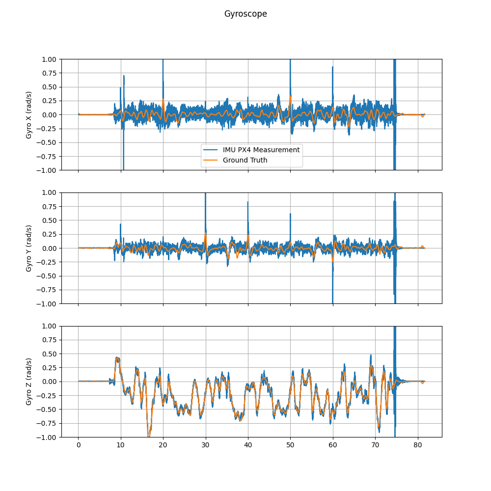
Plotting the IMU measurements is then straightforward. We first plot the angular velocity measurements from the IMU and the ground truth.

axs[0].plot(time, imu_px4["angular_velocity.x"], label="IMU PX4 Measurement")
axs[1].plot(time, imu_px4["angular_velocity.y"], label="IMU PX4 Measurement")
axs[2].plot(time, imu_px4["angular_velocity.z"], label="IMU PX4 Measurement")

axs[0].plot(time, gt_gyro[0, :], label="Ground Truth")
axs[1].plot(time, gt_gyro[1, :], label="Ground Truth")
axs[2].plot(time, gt_gyro[2, :], label="Ground Truth")

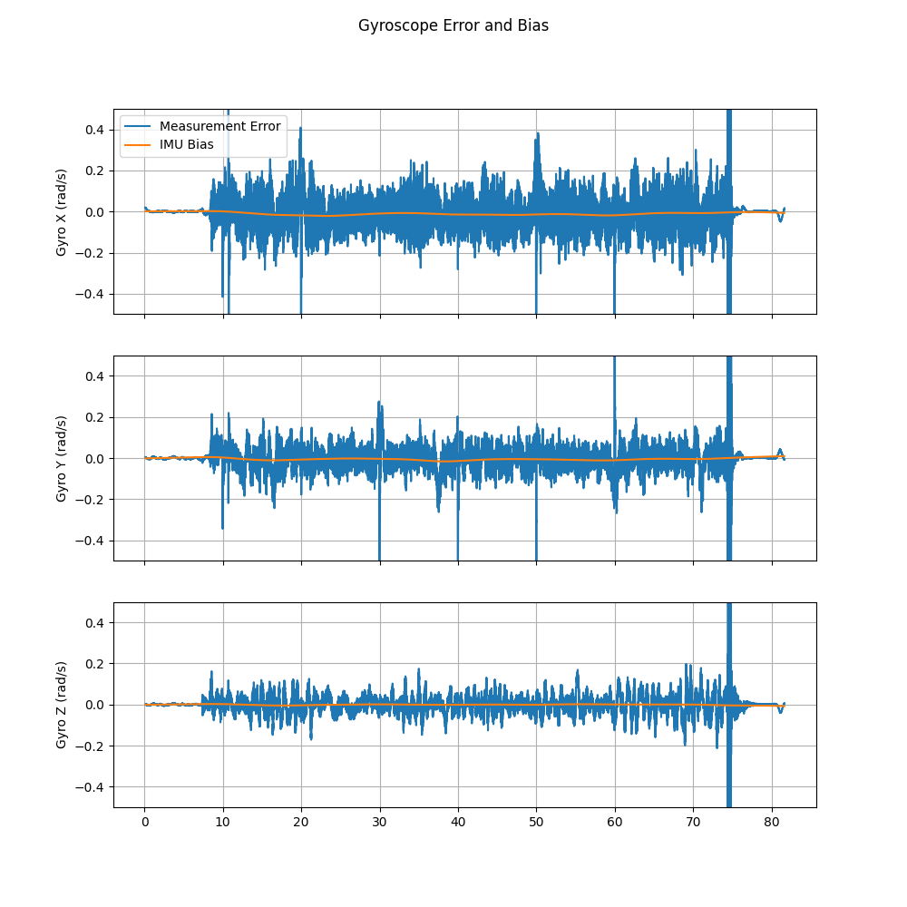
We then plot the measurement error and the compute ground truth bias for the gyroscope measurements.

axs[0].plot(time, gt_gyro[0, :] - imu_px4["angular_velocity.x"], label="Measurement Error")
axs[1].plot(time, gt_gyro[1, :] - imu_px4["angular_velocity.y"], label="Measurement Error")
axs[2].plot(time, gt_gyro[2, :] - imu_px4["angular_velocity.z"], label="Measurement Error")

axs[0].plot(time, imu_px4["gyro_bias.x"], label="IMU Bias")
axs[1].plot(time, imu_px4["gyro_bias.y"], label="IMU Bias")
axs[2].plot(time, imu_px4["gyro_bias.z"], label="IMU Bias")

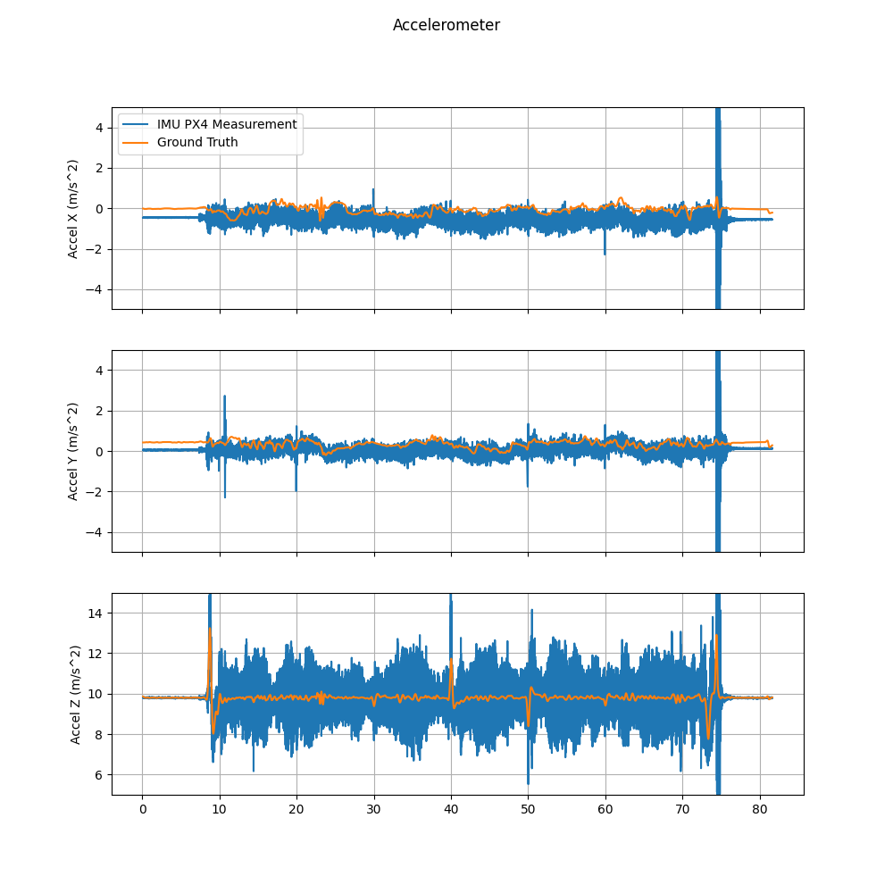
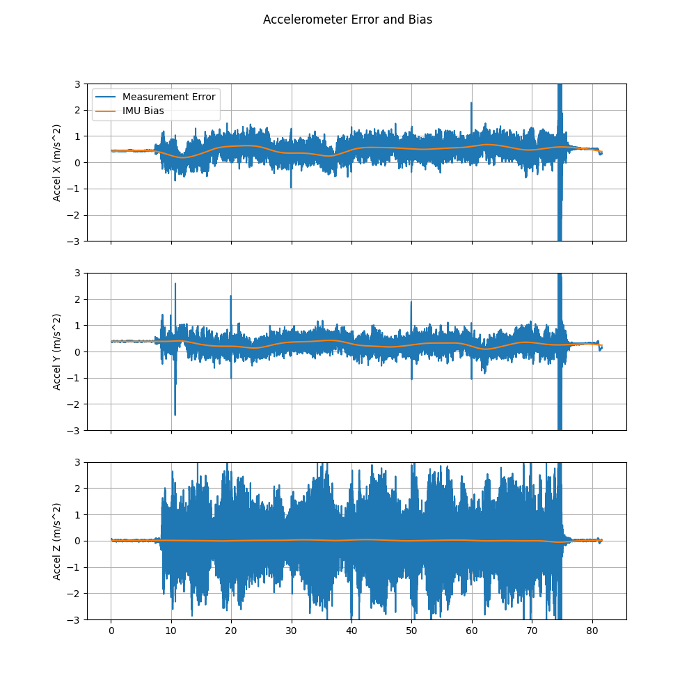
Similarly, we plot the accelerometer measurements, the ground truth, the measurement error, and the computed ground truth bias as follows.

axs[0].plot(time, imu_px4["linear_acceleration.x"], label="IMU PX4 Measurement")
axs[1].plot(time, imu_px4["linear_acceleration.y"], label="IMU PX4 Measurement")
axs[2].plot(time, imu_px4["linear_acceleration.z"], label="IMU PX4 Measurement")

axs[0].plot(time, gt_accelerometer[0, :], label="Ground Truth")
axs[1].plot(time, gt_accelerometer[1, :], label="Ground Truth")
axs[2].plot(time, gt_accelerometer[2, :], label="Ground Truth")

axs[0].plot(time, gt_accelerometer[0, :] - imu_px4["linear_acceleration.x"], label="Measurement Error")
axs[1].plot(time, gt_accelerometer[1, :] - imu_px4["linear_acceleration.y"], label="Measurement Error")
axs[2].plot(time, gt_accelerometer[2, :] - imu_px4["linear_acceleration.z"], label="Measurement Error")

axs[0].plot(time, imu_px4["accel_bias.x"], label="IMU Bias")
axs[1].plot(time, imu_px4["accel_bias.y"], label="IMU Bias")
axs[2].plot(time, imu_px4["accel_bias.z"], label="IMU Bias")