$SE(3)$ EKF with VINS - Three Robots

Overview

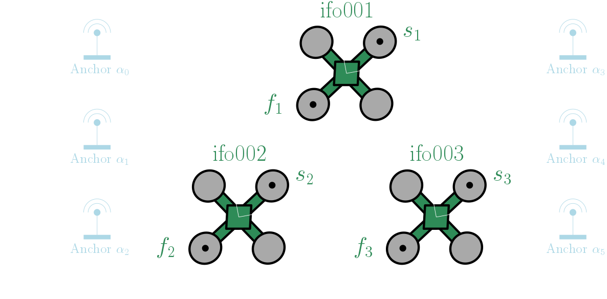
This example shows he we can use MILUV to test out an Extended Kalman Filter (EKF) for three robots using Visual-Inertial Navigation System (VINS) data. This example builds off the one-robot VINS EKF example and extends it to three robots. The setup is similar to the one-robot example, but now we have three robots: ifo001, ifo002, and ifo003. We have the same sensors as the one-robot example, but now we have inter-robot UWB range data.

The state we are trying to estimate is each robot’s 3D pose in the absolute frame, which is represented by

\[\{ \mathbf{T}_{a1}, \mathbf{T}_{a2}, \mathbf{T}_{a3} \} \in SE(3) \times SE(3) \times SE(3),\]

where $\mathbf{T}_{ai}$ is the pose of robot ifo00$i$ in the absolute frame. Similar to the one-robot example, we use $\tau_i \in \{ f_i, s_i \} $ to denote the tag on robot ifo00$i$, and we assume we know the moment arm of tag $\tau_i$ on robot ifo00$i$, which is provided in config/uwb/tags.yaml.

Importing Libraries and MILUV Utilities

As in the one-robot example, we start by importing the necessary libraries and utilities, with the only difference being that we import the three-robot models instead of the one-robot models.

import numpy as np
import pandas as pd

from miluv.data import DataLoader
import miluv.utils as utils
import examples.ekfutils.vins_one_robot_models as model
import examples.ekfutils.common as common

Loading the Data

For this example, we will use experiment 1c, which is a three-robot experiment with VINS data.

exp_name = "1c"

We then, in one line, load all the sensor data we want for our EKF. We keep only the data for this example and get rid of the other functions in the DataLoader class.

miluv = DataLoader(exp_name, imu = "px4", cam = None, mag = False, remove_imu_bias = True)
data = miluv.data

We now extract the VINS data in a similar manner to the one-robot example, but now we do it for all three robots. This approach of dictionary comprehension will be a common theme in adapting the one-robot example to multiple robots.

vins = {robot: utils.load_vins(exp_name, robot, loop = False, postprocessed = True) for robot in data.keys()}

To make the subsequent code similar to the one-robot example, we extract the UWB range and height data for all three robots into a single DataFrame per sensor.

uwb_range = pd.concat([data[robot]["uwb_range"] for robot in data.keys()])
height = pd.concat([data[robot]["height"].assign(robot=robot) for robot in data.keys()])

Then, in a similar manner to the one-robot example, we align the sensor data timestamps to the VINS data timestamps.

query_timestamps = np.append(uwb_range["timestamp"].to_numpy(), height["timestamp"].to_numpy())
query_timestamps = query_timestamps[
    (query_timestamps > vins["ifo001"]["timestamp"].iloc[0]) & (query_timestamps < vins["ifo001"]["timestamp"].iloc[-1]) &
    (query_timestamps > vins["ifo002"]["timestamp"].iloc[0]) & (query_timestamps < vins["ifo002"]["timestamp"].iloc[-1]) &
    (query_timestamps > vins["ifo003"]["timestamp"].iloc[0]) & (query_timestamps < vins["ifo003"]["timestamp"].iloc[-1])
]
query_timestamps = np.sort(np.unique(query_timestamps))

We then use this to query the gyro and VINS data at these timestamps, where we use dictionary comprehension to get the data for all three robots.

imu_at_query_timestamps = {
    robot: miluv.query_by_timestamps(query_timestamps, robots=robot, sensors="imu_px4")[robot]
    for robot in data.keys()
}
gyro: pd.DataFrame = {
    robot: imu_at_query_timestamps[robot]["imu_px4"][["timestamp", "angular_velocity.x", "angular_velocity.y", "angular_velocity.z"]]
    for robot in data.keys()
}
vins_at_query_timestamps = {
    robot: utils.zero_order_hold(query_timestamps, vins[robot]) for robot in data.keys()
}

Then, the ground truth data,

gt_se3 = {
    robot: utils.get_se3_poses(data[robot]["mocap_quat"](query_timestamps), data[robot]["mocap_pos"](query_timestamps)) 
    for robot in data.keys()
}

And lastly, we convert each robot’s VINS data to its own respective body frame.

vins_body_frame = {
    robot: common.convert_vins_velocity_to_body_frame(vins_at_query_timestamps[robot], gt_se3[robot]) 
    for robot in data.keys()
}

Extended Kalman Filter

We now implement the EKF for the three-robot VINS example, which is similar to the one-robot example, but is more involved due to the additional robots and the inter-robot UWB range data.

We start by initializing a variable to store the EKF state and covariance for each robot.

ekf_history = {
    robot: common.MatrixStateHistory(state_dim=4, covariance_dim=6) for robot in data.keys()
}

We then initialize the EKF with the first ground truth pose, the anchor postions, and UWB tag moment arms. As before, inside the constructor of the EKF, we add noise to have some initial uncertainty in the state.

ekf = model.EKF(
    {robot: gt_se3[robot][0] for robot in data.keys()}, 
    miluv.anchors, 
    miluv.tag_moment_arms
)

And now, the EKF loop.

for i in range(0, len(query_timestamps)):
    # ----> TODO: Implement the EKF prediction and correction steps

Prediction

The prediction step is exactly the same as in the one-robot example, but now we do it for all three robots using each robot’s interoceptive data. In the code, we generate the input vector for each robot using

for i in range(0, len(query_timestamps)):
    input = {
        robot: np.array([
            gyro[robot].iloc[i]["angular_velocity.x"], gyro[robot].iloc[i]["angular_velocity.y"], 
            gyro[robot].iloc[i]["angular_velocity.z"], vins_body_frame[robot].iloc[i]["twist.linear.x"],
            vins_body_frame[robot].iloc[i]["twist.linear.y"], vins_body_frame[robot].iloc[i]["twist.linear.z"],
        ])
        for robot in data.keys()
    }

    # ----> TODO: EKF prediction using the gyro and vins data

Then, as before, we abstract the prediction step by calling the predict method of the EKF, which is implemented in the models module.

for i in range(0, len(query_timestamps)):
    # .....
    
    # Do an EKF prediction using the gyro and vins data
    dt = (query_timestamps[i] - query_timestamps[i - 1]) if i > 0 else 0
    ekf.predict(input, dt)

Correction

The UWB correction for the multi-robot case looks exactly the same as the one-robot case in the main script, and can be performed by running the following code.

# Iterate through the query timestamps
for i in range(0, len(query_timestamps)):
    # .....

    # Check if range data is available at this query timestamp, and do an EKF correction
    range_idx = np.where(uwb_range["timestamp"] == query_timestamps[i])[0]
    if len(range_idx) > 0:
        range_data = uwb_range.iloc[range_idx]
        ekf.correct({
            "range": float(range_data["range"].iloc[0]),
            "to_id": int(range_data["to_id"].iloc[0]),
            "from_id": int(range_data["from_id"].iloc[0])
        })

However, under the hood in the models module, this is a bit more involved. We have to check if the range data is between a robot and an anchor or between two robots. The models for the former is pretty much exactly the same as the one-code case. Meanwhile, for the latter, the measurement model is given by

\[y = \lVert \mathbf{r}_a^{\tau_i \tau_j} \rVert,\]

which can be written as

\[y = \lVert (\mathbf{C}_{ai} \mathbf{r}_i^{\tau_i i} + \mathbf{r}_a^{ia}) - (\mathbf{C}_{aj} \mathbf{r}_j^{\tau_j j} + \mathbf{r}_a^{ja}) \rVert.\]

It can be shown that this can be written as a function of the state using

\[y = \lVert \hspace{1pt} \boldsymbol{\Pi} ( \mathbf{T}_{ai} \mathbf{\tilde{r}}_{i}^{\tau_i i} - \mathbf{T}_{aj} \mathbf{\tilde{r}}_{j}^{\tau_j j} ) \hspace{1pt} \rVert\]

where, as before,

\[\boldsymbol{\Pi} = \begin{bmatrix} \mathbf{1}_3 & \mathbf{0}_{3 \times 1} \end{bmatrix} \in \mathbb{R}^{3 \times 4}, \qquad \mathbf{\tilde{r}}_{i}^{\tau_i i} = \begin{bmatrix} \mathbf{r}_i^{\tau_i i} \\ 1 \end{bmatrix} \in \mathbb{R}^4.\]

The resemblence to the one-robot case is clear, and we will see the similarity in the Jacobian as well. By defining

\[\boldsymbol{\nu} = \boldsymbol{\Pi} ( \mathbf{T}_{ai} \mathbf{\tilde{r}}_{i}^{\tau_i i} - \mathbf{T}_{aj} \mathbf{\tilde{r}}_{j}^{\tau_j j} ),\]

the Jacobian of the measurement model with respect to the state is given by

\[\delta y = \frac{\boldsymbol{\nu}^\intercal}{\lVert \boldsymbol{\nu} \rVert} \boldsymbol{\Pi} \bar{\mathbf{T}}_{ai} (\mathbf{\tilde{r}}_{i}^{\tau_i i})^\odot \delta \boldsymbol{\xi}_i - \frac{\boldsymbol{\nu}^\intercal}{\lVert \boldsymbol{\nu} \rVert} \boldsymbol{\Pi} \bar{\mathbf{T}}_{aj} (\mathbf{\tilde{r}}_{j}^{\tau_j j})^\odot \delta \boldsymbol{\xi}_j,\]

where, as before, $(\cdot)^\odot : \mathbb{R}^4 \rightarrow \mathbb{R}^{4 \times 6}$ is the odot operator in $SE(3)$.

The height correction is also the same as the one-robot case, and can be performed by running the following code.

for i in range(0, len(query_timestamps)):
    # .....

    # Check if height data is available at this query timestamp, and do an EKF correction
    height_idx = np.where(height["timestamp"] == query_timestamps[i])[0]
    if len(height_idx) > 0:
        height_data = height.iloc[height_idx]
        ekf.correct({
            "height": float(height_data["range"].iloc[0]),
            "robot": height_data["robot"].iloc[0]
        })

Lastly, we store the EKF state and covariance at this query timestamp for postprocessing.

for i in range(0, len(query_timestamps)):
    # .....

    for robot in data.keys():
    ekf_history[robot].add(query_timestamps[i], ekf.x[robot], ekf.get_covariance(robot))

Results

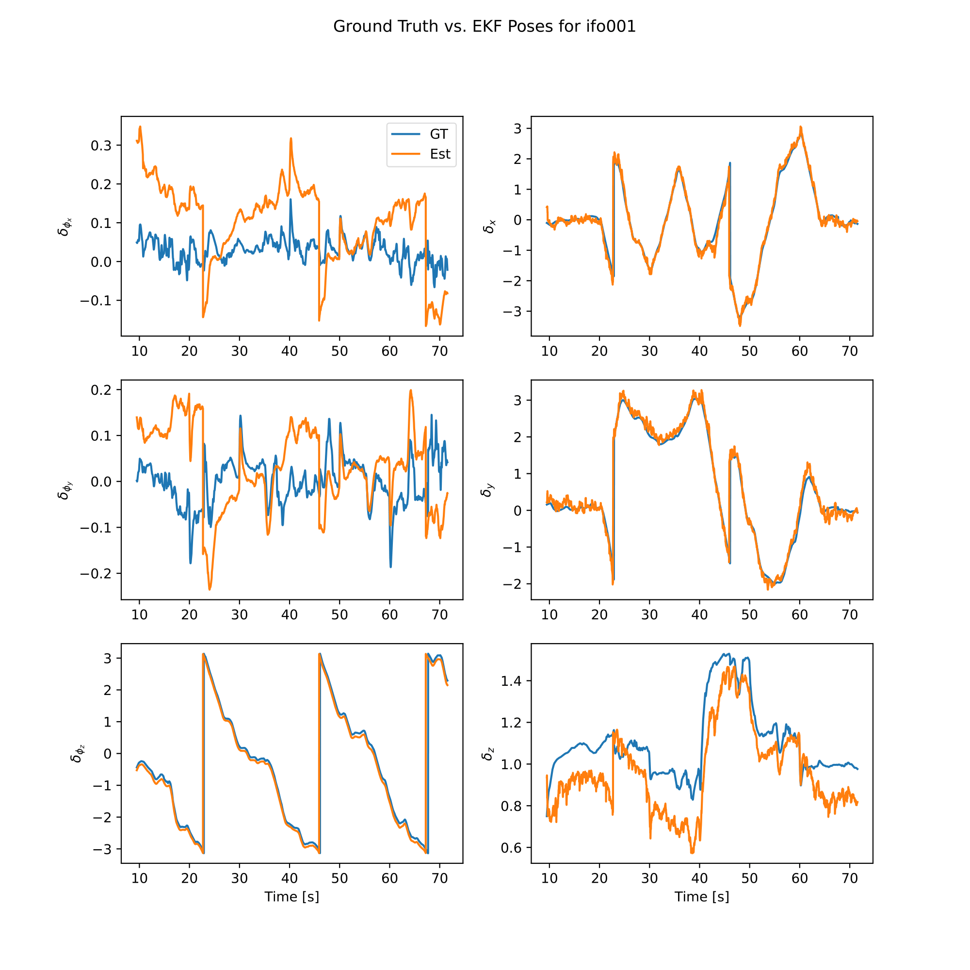
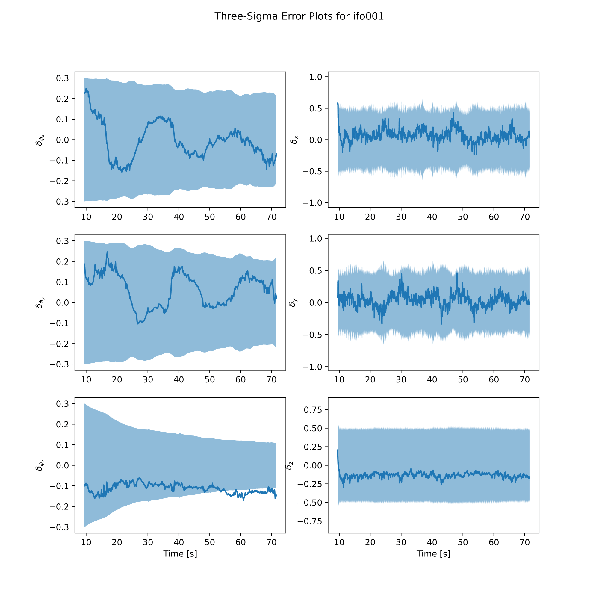
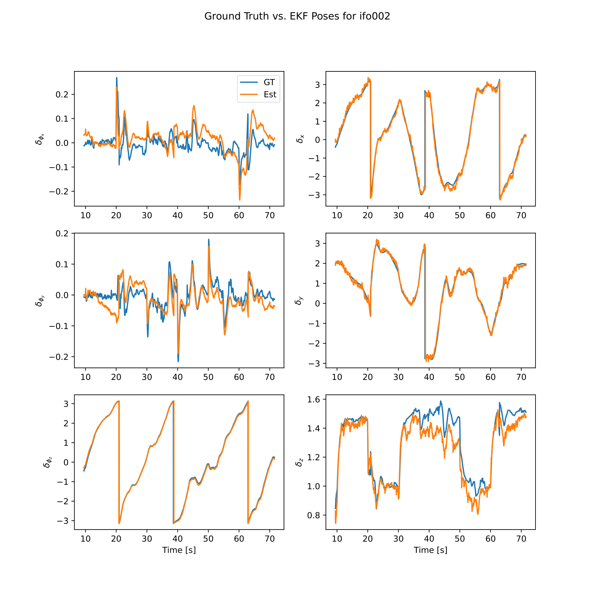
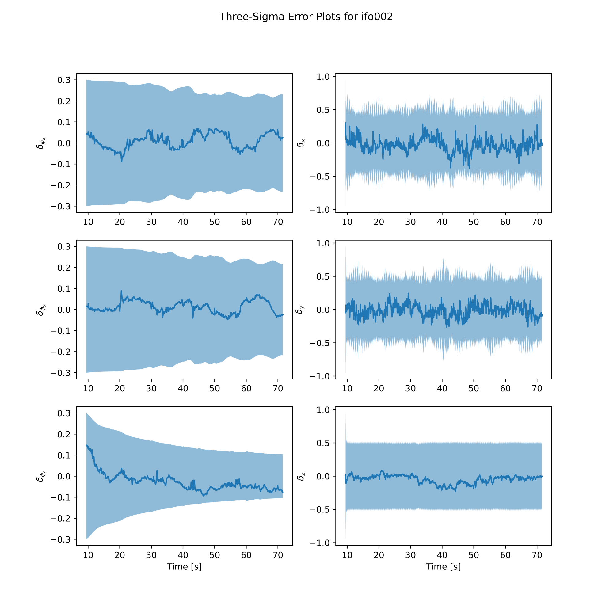
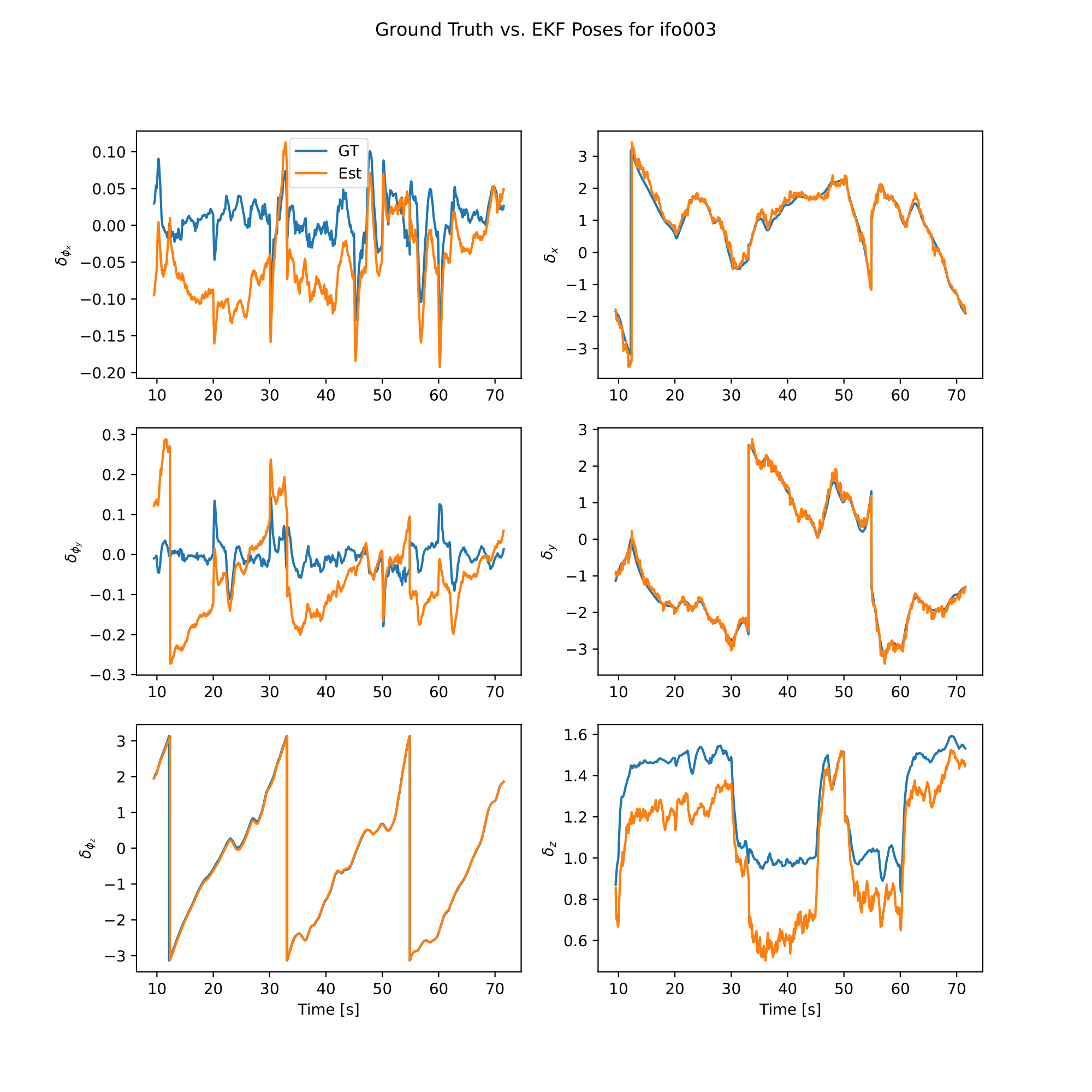
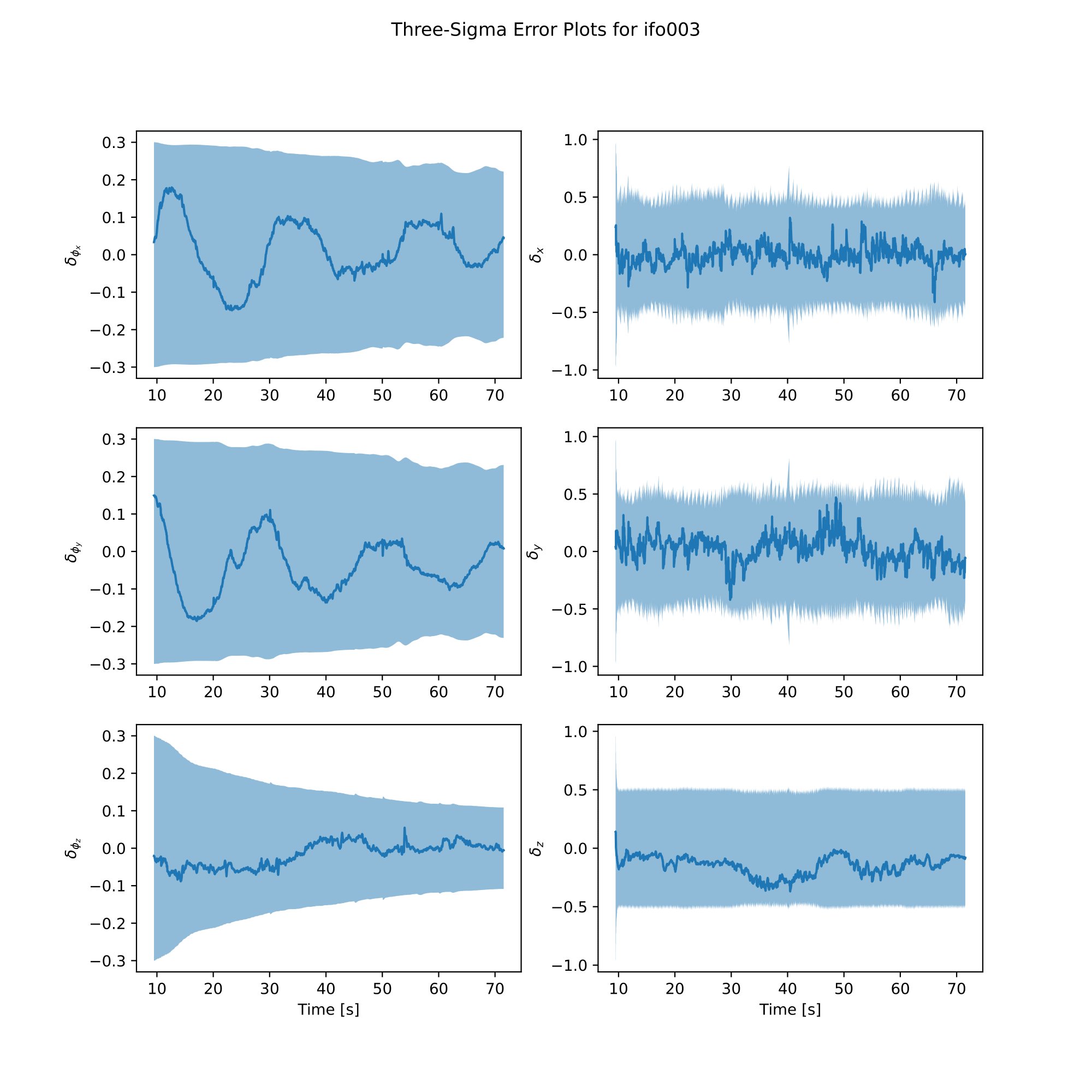
To run the evaluation of the EKF, we run the code as the one-robot example, and now we are done!

analysis = model.EvaluateEKF(gt_se3, ekf_history, exp_name)

analysis.plot_error()
analysis.plot_poses()
analysis.save_results()