$SE_2(3)$ EKF with IMU - One Robot

This example shows how we can use MILUV to test out an Extended Kalman Filter (EKF) for a single robot using an Inertial Measurement Unit (IMU). The derivations here are a little bit more involved than the VINS EKF example, but we’ll show that the EKF implementation is still straightforward using the MILUV devkit. Nonetheless, we suggest looking at the VINS example first before proceeding with this one. In this example, we will use the following data:
- Gyroscope and accelerometer data from the robot’s PX4 IMU.
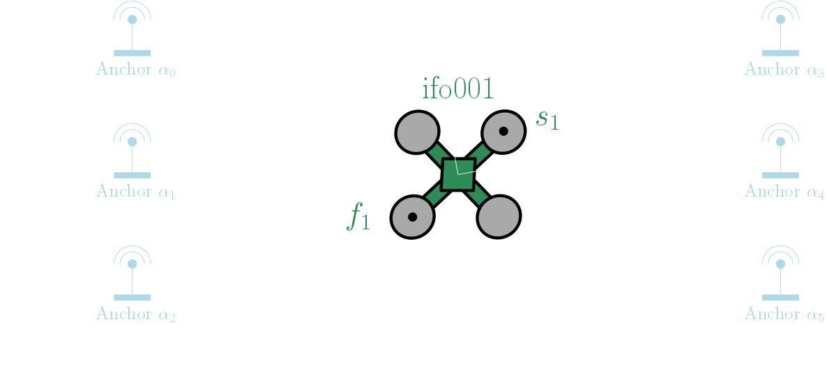
- UWB range data between the 2 tags on the robot and the 6 anchors in the environment.
- Height data from the robot’s downward-facing laser rangefinder.
- Ground truth pose data from a motion capture system to evaluate the EKF.
The state we are trying to estimate is the robot’s 3D pose in the absolute frame, which is represented by
\[\mathbf{T}_{a1} = \begin{bmatrix} \mathbf{C}_{a1} & \mathbf{v}^{1a}_a & \mathbf{r}^{1a}_a \\ \mathbf{0} & 1 & 0 \\ 0 & 0 & 1 \end{bmatrix} \in SE_2(3).\]In this example, we also estimate the gyroscope and accelerometer biases, which are represented by
\[\boldsymbol{\beta} = \begin{bmatrix} \boldsymbol{\beta}^\text{gyr} \\ \boldsymbol{\beta}^\text{acc} \end{bmatrix} \in \mathbb{R}^6.\]We follow the same notation convention mentioned in the paper and assume the same assumptions introduced in the VINS EKF example.
Importing Libraries and MILUV Utilities
We start by importing the necessary libraries and utilities for this example as in the VINS example, with the only change being the EKF model we are using.
import numpy as np
import pandas as pd

from miluv.data import DataLoader
import miluv.utils as utils
import examples.ekfutils.imu_one_robot_models as model
import examples.ekfutils.common as common
Loading the Data
We will use the same experiment as in the VINS example, and load only ifo001’s data for this example.
exp_name = "default_1_random3_0"

miluv = DataLoader(exp_name, imu = "px4", cam = None, mag = False)
data = miluv.data["ifo001"]
We then extract all timestamps where exteroceptive data is available.
query_timestamps = np.append(
    data["uwb_range"]["timestamp"].to_numpy(), data["height"]["timestamp"].to_numpy()
)
query_timestamps = np.sort(np.unique(query_timestamps))
We then use this to query the IMU data at these timestamps, extracing both the accelerometer and gyroscope data.
imu_at_query_timestamps = miluv.query_by_timestamps(query_timestamps, robots="ifo001", sensors="imu_px4")["ifo001"]
accel: pd.DataFrame = imu_at_query_timestamps["imu_px4"][["timestamp", "linear_acceleration.x", "linear_acceleration.y", "linear_acceleration.z"]]
gyro: pd.DataFrame = imu_at_query_timestamps["imu_px4"][["timestamp", "angular_velocity.x", "angular_velocity.y", "angular_velocity.z"]]
To be able to evaluate our EKF, we extract the ground truth pose data at these timestamps. The DataLoader class provides interpolated splines for the ground truth pose data, and the reason for that is that we can query the ground truth data at any timestamp and call the derivative method to get higher-order derivatives of the pose data. For example, here we use the first derivative of the pose data to get the linear velocity data, which is necessary to evaluate our $SE_2(3)$ EKF. We use a helper function from the utils module to convert the mocap pose data and its derivatives to a list of $SE_2(3)$ poses.
gt_se23 = utils.get_se23_poses(
    data["mocap_quat"](query_timestamps), data["mocap_pos"].derivative(nu=1)(query_timestamps), data["mocap_pos"](query_timestamps)
)
Additionally, we extract the IMU biases at these timestamps to evaluate the EKF’s bias estimates. These ground truth biases are provided as part of the dataset, and are computed by comparing the smoothed IMU data with the ground truth pose data.
gt_bias = imu_at_query_timestamps["imu_px4"][[
    "gyro_bias.x", "gyro_bias.y", "gyro_bias.z",
    "accel_bias.x", "accel_bias.y", "accel_bias.z"
]].to_numpy()
Extended Kalman Filter
We now implement the EKF for the one-robot IMU example. In here, we will go through some of the implementation details of the EKF, but as before, the EKF implementation is in the models module and the main script only calls these EKF methods to avoid cluttering the main script.
We start by initializing a variable to store the EKF state and covariance at each query timestamp for postprocessing. Given that the state is composed of a matrix component (the pose) and a vector component (the bias), we initialize two state histories to store the pose and bias components.
ekf_history = {
    "pose": common.MatrixStateHistory(state_dim=5, covariance_dim=9),
    "bias": common.VectorStateHistory(state_dim=6)
}
We then initialize the EKF with the first ground truth pose, the anchor positions, and UWB tag moment arms. Inside the constructor of the EKF, we add noise to have some initial uncertainty in the state, and set the initial bias estimate to zero.
ekf = model.EKF(gt_se23[0], miluv.anchors, miluv.tag_moment_arms)
The main loop of the EKF is to iterate through the query timestamps and do the prediction and correction steps, which is where the EKF magic happens and is what we will go through next.
for i in range(0, len(query_timestamps)):
    # ----> TODO: Implement the EKF prediction and correction steps
Prediction
The prediction step is done using the IMU data, where the gyroscope reads a biased angular velocity
\[\mathbf{u}^\text{gyr} = \boldsymbol{\omega}^{1a}_1 - \boldsymbol{\beta}^\text{gyr} - \mathbf{w}^\text{gyr},\]and the accelerometer reads a biased specific force
\[\mathbf{u}^\text{acc} = \mathbf{a}^{1a}_1 - \boldsymbol{\beta}^\text{acc} - \mathbf{w}^\text{acc},\]where $\mathbf{w}^\text{gyr}$ and $\mathbf{w}^\text{acc}$ are the white noise terms for the gyroscope and accelerometer, respectively, and $\boldsymbol{\omega}^{1a}_1$ and $\mathbf{a}^{1a}_1$ are the angular velocity and linear acceleration, respectively, in the robot’s body frame. In the code, we extract the IMU data at the current query timestamp as follows:
for i in range(0, len(query_timestamps)):
    input = np.array([
        gyro.iloc[i]["angular_velocity.x"], gyro.iloc[i]["angular_velocity.y"],
        gyro.iloc[i]["angular_velocity.z"], accel.iloc[i]["linear_acceleration.x"],
        accel.iloc[i]["linear_acceleration.y"], accel.iloc[i]["linear_acceleration.z"]
    ])

    # ----> TODO: EKF prediction using the gyro and vins data
The subsequent derivation is a little bit involved and we skip through a lot of the details for brevity, but for a more detailed derivation of the process model, one can refer to Chapter 9 in the book State Estimation for Robotics, Second Edition by Timothy D. Barfoot.
The continuous-time process model for the orientation is given by
\[\dot{\mathbf{ C }}_{a1} = \mathbf{C}_{a1} (\boldsymbol{\omega}^{1a} _ 1)^{\wedge},\]where $(\cdot)^{\wedge}$ is the skew-symmetric matrix operator in that maps an element of $\mathbb{R}^3$ to the Lie algebra of $SO(3)$. Meanwhile, the continuous-time process model for the velocity is given by
\[\dot{\mathbf{v}}^{1a}_a = \mathbf{C}_{a1} \mathbf{a}^{1a}_1 + \mathbf{g}_a,\]where $\mathbf{g}_a$ is the gravity vector in the absolute frame. The continuous-time process model for the position is given by
\[\dot{\mathbf{r}}^{1a}_a = \mathbf{v}^{1a}_a.\]We can show that the continuous-time process model for the state $\mathbf{T}_{a1}$ can be written compactly as
\[\dot{\mathbf{T}}_{a1} = \mathbf{T}_{a1} \mathbf{U} + \mathbf{G} \mathbf{T}_{a1},\]where
\[\mathbf{U} = \begin{bmatrix} (\boldsymbol{\omega}^{1a}_1)^\wedge & \mathbf{a}^{1a}_1 & \\ & & 1 \\ & & 0 \end{bmatrix} \in \mathbb{R}^{5 \times 5}, \qquad \mathbf{G} = \begin{bmatrix} \mathbf{0} & \mathbf{g}_a & \\ & & -1 \\ & & 0 \end{bmatrix} \in \mathbb{R}^{5 \times 5}.\]To implement the prediction step in an EKF, we first discretize the continuous-time process model over a timestep $\Delta t$ using the matrix exponential to yield
\[\begin{aligned} \mathbf{T}_{a1,k+1} &= \operatorname{exp} (\Delta t \mathbf{G}) \mathbf{T}_{a1,k} \operatorname{exp} (\Delta t \mathbf{U}) \\ &\triangleq \mathbf{G}_k \mathbf{T}_{a1,k} \mathbf{U}_k, \end{aligned}\]where
\[\begin{aligned} \mathbf{G}_k &= \begin{bmatrix} \mathbf{1} & \Delta t \mathbf{g}_a & - \frac{1}{2} \Delta t^2 \mathbf{g}_a \\ & 1 & - \Delta t \\ & & 1 \end{bmatrix}, \\ \mathbf{U}_k &= \begin{bmatrix} \operatorname{Exp} (\Delta t \boldsymbol{\omega}) & \Delta t \mathbf{J}_l(\Delta t \boldsymbol{\omega}) \mathbf{a} & \frac{1}{2} \Delta t^2 \mathbf{N}( \Delta t \boldsymbol{\omega}) \mathbf{a} \\ & 1 & \Delta t \\ & & 1 \end{bmatrix}, \end{aligned}\]where $\operatorname{Exp} (\cdot)$ is the operator that maps an element of $\mathbb{R}^3$ to $SO(3)$, $\mathbf{J}_l(\cdot)$ is the left Jacobian of $SO(3)$, and $\mathbf{N}(\cdot)$ is defined in Appendix C of this paper. Note that the subscripts and superscripts have been dropped from the inputs for brevity.
By perturbing the state and inputs in a similar manner as in the VINS example, we can show that the linearized process model for the pose state is given by
\[\delta \boldsymbol{\xi}_{k+1} = \operatorname{Ad} (\mathbf{U}_{k-1}^{-1}) \delta \boldsymbol{\xi}_k - \mathbf{L}_{k} \delta \boldsymbol{\beta}_k + \mathbf{L}_k \delta \mathbf{w}_k,\]where $\operatorname{Ad} (\cdot)$ is the Adjoint matrix in $SE_2(3)$,
\[\mathbf{L}_k = \mathscr{J} \left( - \begin{bmatrix} \Delta t \boldsymbol{\omega} \\ \Delta t \mathbf{a} \\ \frac{1}{2} \Delta t^2 \mathbf{J}_l(\Delta t \boldsymbol{\omega})^{-1} \mathbf{N}(\Delta t \boldsymbol{\omega}) \mathbf{a} \end{bmatrix} \right) \begin{bmatrix} \Delta t \mathbf{1} & 0 \\ 0 & \Delta t \mathbf{1} \\ \Delta t^3 (\frac{1}{12} \mathbf{1}^\wedge - \frac{1}{720} \Delta t^2 \mathbf{M}) & \frac{1}{2} \Delta t^2 \mathbf{J}_l(\Delta t \boldsymbol{\omega})^{-1} \mathbf{N}(\Delta t \boldsymbol{\omega}) \end{bmatrix},\]$\mathscr{J}(\cdot)$ is the left Jacobian in $SE_2(3)$, and $\mathbf{M}$ is defined as
\[\mathbf{M} = \boldsymbol{\omega}^\wedge \boldsymbol{\omega}^\wedge \mathbf{a}^\wedge + \boldsymbol{\omega}^\wedge (\boldsymbol{\omega}^\wedge \mathbf{a})^\wedge + (\boldsymbol{\omega}^\wedge \boldsymbol{\omega}^\wedge \mathbf{a})^\wedge.\]This summarizes the prediction step for the pose states. Meanwhile, the prediction step for the bias states is given by a random walk model
\[\dot{\boldsymbol{\beta}} = \mathbf{w},\]where $\mathbf{w}$ is the white noise term for the bias states. This can be simply discretized as
\[\boldsymbol{\beta}_{k+1} = \boldsymbol{\beta}_k + \Delta t \mathbf{w}_k,\]and given that this is a linear model, the Jacobians are simply the identity matrix.
As before, the process model and the Jacobians are implemented in the models module, and as such the prediction step boils down to simply calling the predict method of the EKF.
for i in range(0, len(query_timestamps)):
    # .....

    # Do an EKF prediction using the gyro and vins data
    dt = (query_timestamps[i] - query_timestamps[i - 1]) if i > 0 else 0
    ekf.predict(input, dt)
Also as before, we set the process model covariances using the get_imu_noise_params() function in the miluv.utils module, which reads the robot-specific IMU noise and bias parameters from the config/imu folder that were extracted using the allan_variance_ros package.
Correction
The correction models for the UWB range and height data are almost identical to the VINS EKF example, so we will skip through this section. The only difference for the UWB range is that $\boldsymbol{\Pi}$ and $\mathbf{\tilde{r}}_{1}^{\tau_1 1}$ are defined as
\[\boldsymbol{\Pi} = \begin{bmatrix} \mathbf{1}_3 & \mathbf{0}_{3 \times 2} \end{bmatrix} \in \mathbb{R}^{3 \times 5}, \qquad \mathbf{\tilde{r}}_{1}^{\tau_1 1} = \begin{bmatrix} \mathbf{r}_1^{\tau_1 1} \\ 0 \\ 1 \end{bmatrix} \in \mathbb{R}^5,\]and the $\odot$ operator used in the Jacobian is the odot operator in $SE_2(3)$.
# Iterate through the query timestamps
for i in range(0, len(query_timestamps)):
    # .....

    # Check if range data is available at this query timestamp, and do an EKF correction
    range_idx = np.where(data["uwb_range"]["timestamp"] == query_timestamps[i])[0]
    if len(range_idx) > 0:
        range_data = data["uwb_range"].iloc[range_idx]
        ekf.correct({
            "range": float(range_data["range"].iloc[0]),
            "to_id": int(range_data["to_id"].iloc[0]),
            "from_id": int(range_data["from_id"].iloc[0])
        })
Meanwhile, the only difference for the height data is that $\mathbf{a}$ and $\mathbf{b}$ are defined as
\[\mathbf{a} = \begin{bmatrix} 0 \\ 0 \\ 1 \\ 0 \\ 0 \end{bmatrix}, \qquad \mathbf{b} = \begin{bmatrix} 0 \\ 0 \\ 0 \\ 0 \\ 1 \end{bmatrix}.\]for i in range(0, len(query_timestamps)):
# .....
# Check if height data is available at this query timestamp, and do an EKF correction
height_idx = np.where(data["height"]["timestamp"] == query_timestamps[i])[0]
if len(height_idx) > 0:
height_data = data["height"].iloc[height_idx]
ekf.correct({"height": float(height_data["range"].iloc[0])})
Lastly, we store the EKF state and covariance at this query timestamp for postprocessing.
for i in range(0, len(query_timestamps)):
    # .....

    # Store the EKF state and covariance at this query timestamp
    ekf_history["pose"].add(query_timestamps[i], ekf.pose, ekf.pose_covariance)
    ekf_history["bias"].add(query_timestamps[i], ekf.bias, ekf.bias_covariance)
Results
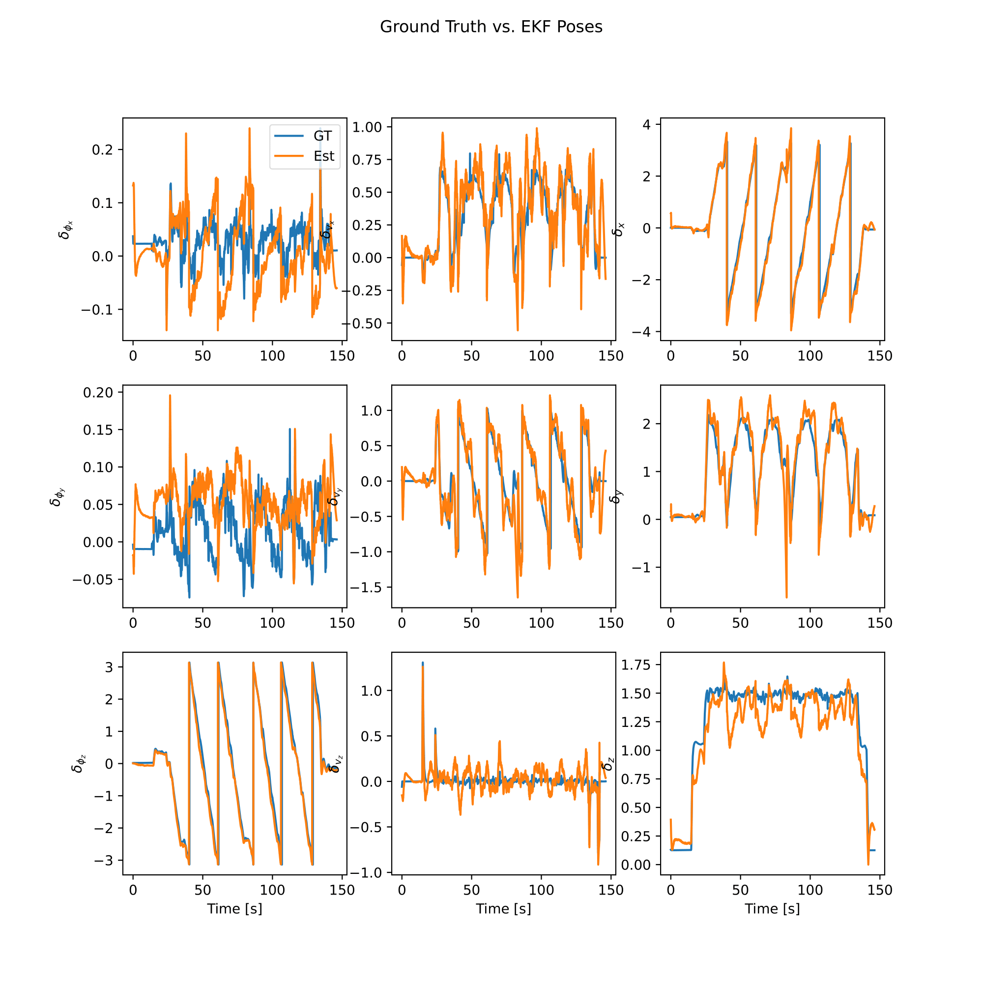
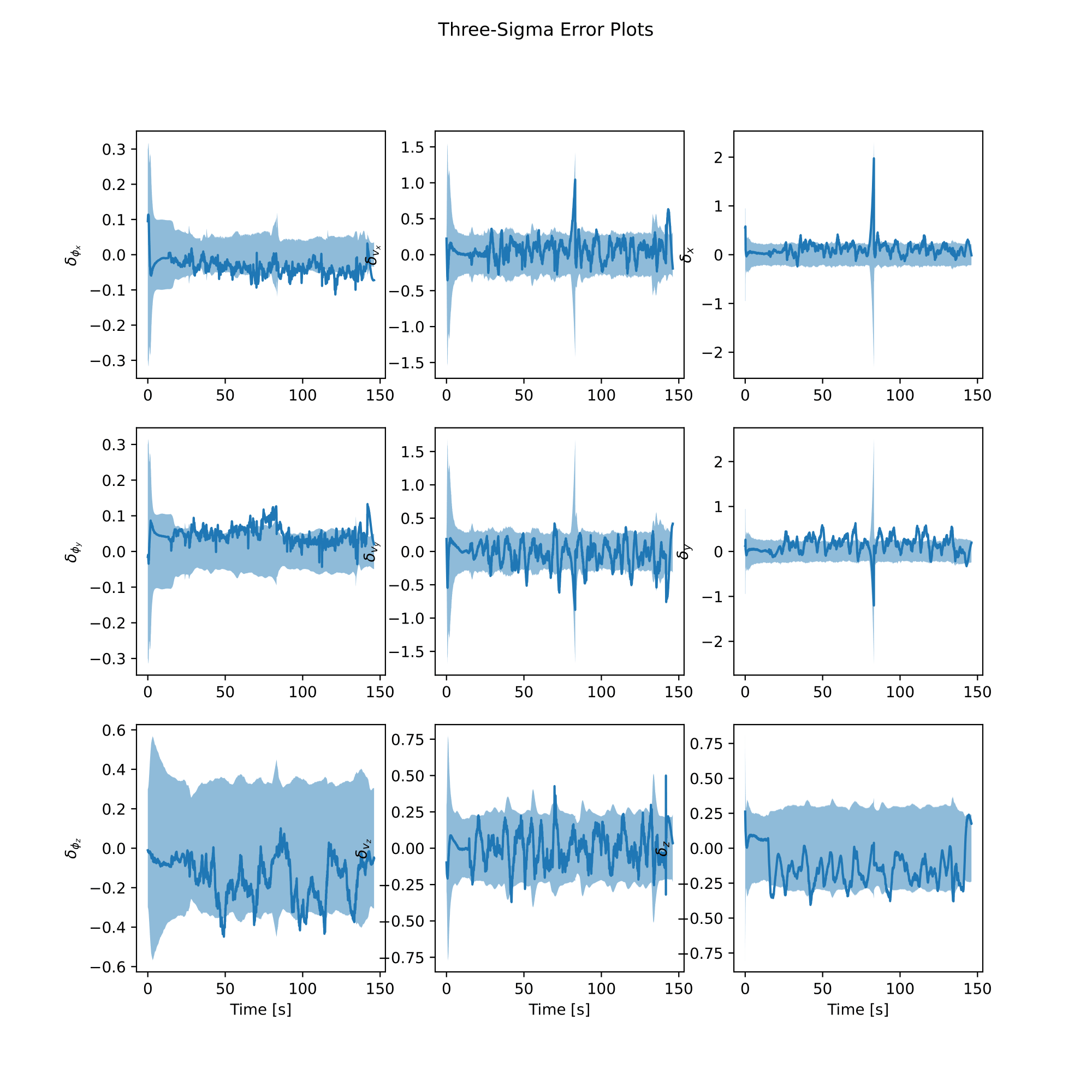
We can now evaluate the EKF using the ground truth data and plot the results. We first evaluate the EKF using the ground truth data and the EKF history, using the example-specific evaluation functions in the models module.
analysis = model.EvaluateEKF(gt_se23, gt_bias, ekf_history, exp_name)
Lastly, we call the following functions to plot the results and save the results to disk, and we are done!
analysis.plot_error()
analysis.plot_poses()
analysis.plot_bias_error()
analysis.save_results()
 |  |