$SE(3)$ EKF with VINS - One Robot
Overview

This example shows he we can use MILUV to test out an Extended Kalman Filter (EKF) for a single robot using Visual-Inertial Navigation System (VINS) data. In this example, we will use the following data:
- Gyroscope data from the robot’s PX4 IMU, where we remove the gyro bias for this example.
- VINS data, which uses the robot’s camera and IMU to estimate the robot’s velocity.
- UWB range data between the 2 tags on the robot and the 6 anchors in the environment.
- Height data from the robot’s downward-facing laser rangefinder.
- Ground truth pose data from a motion capture system to evaluate the EKF.
The state we are trying to estimate is the robot’s 3D pose in the absolute frame, which is represented by
\[\mathbf{T}_{a1} = \begin{bmatrix} \mathbf{C}_{a1} & \mathbf{r}^{1a}_a \\ \mathbf{0} & 1 \end{bmatrix} \in SE(3).\]We follow the same notation convention as mentioned in the paper, and the reference frame ${ F_1 }$ is the body-fixed reference frame of robot ifo001.
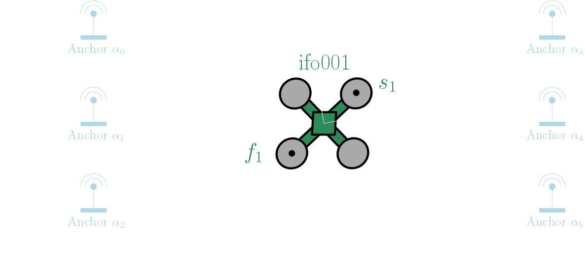
As shown in the figure above, the robot has two UWB tags, $f_1$ and $s_1$, for which we define $\tau_1 \in \{ f_1, s_1 \}$. The robot also has 6 anchors in the environment, which are assumed to be stationary and their positions $ \mathbf{r}^{\alpha_i a}_a \in \mathbb{R}^3 $ are known in the absolute frame as provided in config/uwb/anchors.yaml. Similarly, the moment arm of the tags on the robot, $ \mathbf{r}^{\tau_1 1}_1 \in \mathbb{R}^3 $, is also known and provided in config/uwb/tags.yaml.
Importing Libraries and MILUV Utilities
We start by importing the necessary libraries and utilities for this example. Firstly, we import the standard libraries numpy and pandas for numerical computations and data manipulation.
import numpy as np
import pandas as pd
We then import the DataLoader class from the miluv package, which provides an easy way to load the MILUV dataset. This is the core of the MILUV devkit, and it provides an interface to load the sensor data and ground truth data for the experiments.
from miluv.data import DataLoader
We also import the utils module from the miluv package, which provide utilities for Lie groups that accompany and other helper functions.
import miluv.utils as utils
Each EKF example is accompanied by a models module that contains the EKF implementation for that example to hide the implementation details from the main script. This is since the process model, measurement model, jacobians, and evaluation functions specific for the EKF example are irrelevant to showcase how MILUV can be used. Additionally, the common module contains utility functions that are shared across all EKF examples. We import these to the main script.
import examples.ekfutils.vins_one_robot_models as model
import examples.ekfutils.common as common
Loading the Data
We start by defining the experiment we want to run the EKF on. In this case, we will use experiment default_1_random3_0.
exp_name = "default_1_random3_0"
We then, in one line, load all the sensor data we want for our EKF. For this example, we only care about ifo001’s data, and we remove the IMU bias to simplify the EKF implementation.
miluv = DataLoader(exp_name, imu = "px4", cam = None, mag = False, remove_imu_bias = True)
data = miluv.data["ifo001"]
Additionally, we load the VINS data for ifo001, where we set loop = False to avoid loading the loop-closed VINS data, and postprocessed = True to load the VINS data that has been aligned with the mocap reference frame.
vins = utils.load_vins(exp_name, "ifo001", loop = False, postprocessed = True)
We then extract all timestamps where exteroceptive data is available and within the time range of the VINS data.
query_timestamps = np.append(
    data["uwb_range"]["timestamp"].to_numpy(), data["height"]["timestamp"].to_numpy()
)
query_timestamps = query_timestamps[query_timestamps > vins["timestamp"].iloc[0]]
query_timestamps = query_timestamps[query_timestamps < vins["timestamp"].iloc[-1]]
query_timestamps = np.sort(np.unique(query_timestamps))
We then use this to query the gyro and VINS data at these timestamps.
imu_at_query_timestamps = miluv.query_by_timestamps(query_timestamps, robots="ifo001", sensors="imu_px4")["ifo001"]
gyro: pd.DataFrame = imu_at_query_timestamps["imu_px4"][["timestamp", "angular_velocity.x", "angular_velocity.y", "angular_velocity.z"]]
vins_at_query_timestamps = utils.zero_order_hold(query_timestamps, vins)
To be able to evaluate our EKF, we extract the ground truth pose data at these timestamps. The DataLoader class provides interpolated splines for the ground truth pose data, which we can use to get the ground truth poses at the query timestamps. We use a helper function from the utils module to convert the mocap pose data to a list of $SE(3)$ poses.
gt_se3 = utils.get_se3_poses(
    data["mocap_quat"](query_timestamps), data["mocap_pos"](query_timestamps)
)
Lastly, we convert the VINS data from the absolute (mocap) frame to the robot’s body frame using the ground truth data, such that we can have interoceptive data in the robot’s body frame. This is a bit of a hack to simplify this EKF implementation.
vins_body_frame = common.convert_vins_velocity_to_body_frame(vins_at_query_timestamps, gt_se3)
Extended Kalman Filter
We now implement the EKF for the one-robot VINS example. In here, we will go through some of the implementation details of the EKF, but this is to reiterate that the EKF implementation is in the models module and the main script only calls these EKF methods to avoid cluttering the main script.
We start by initializing a variable to store the EKF state and covariance at each query timestamp for postprocessing.
ekf_history = common.MatrixStateHistory(state_dim=4, covariance_dim=6)
We then initialize the EKF with the first ground truth pose, the anchor postions, and UWB tag moment arms. Inside the constructor of the EKF, we add noise to have some initial uncertainty in the state.
ekf = model.EKF(gt_se3[0], miluv.anchors, miluv.tag_moment_arms)
The main loop of the EKF is to iterate through the query timestamps and do the prediction and correction steps, which is where the EKF magic happens and is what we will go through next.
for i in range(0, len(query_timestamps)):
    # ----> TODO: Implement the EKF prediction and correction steps
Prediction
The prediction step is done using the gyroscope and VINS data. The continuous-time process model for the orientation is given by
\[\dot{\mathbf{ C }}_{a1} = \mathbf{C}_{a1} (\boldsymbol{\omega}^{1a} _ 1)^{\wedge},\]where $\boldsymbol{\omega}^{1a} _ 1$ is the angular velocity measured by the gyroscope, and $(\cdot)^{\wedge}$ is the skew-symmetric matrix operator in that maps an element of $\mathbb{R}^3$ to the Lie algebra of $SO(3)$. Meanwhile, the continuous-time process model for the position is given by
\[\dot{\mathbf{r}}^{1a}_a = \mathbf{C}_{a1} \mathbf{v}^{1a}_1,\]where $\mathbf{v}^{1a}_1$ is the linear velocity measured by VINS after being transformed to the robot’s body frame. By defining the input vector as
\[\mathbf{u} = \begin{bmatrix} \boldsymbol{\omega}^{1a}_1 \\ \mathbf{v}^{1a}_1 \end{bmatrix},\]the continuous-time process model for the state $\mathbf{T}_{a1}$ can be written compactly as
\[\dot{\mathbf{T}}_{a1} = \mathbf{T}_{a1} \mathbf{u}^{\wedge},\]where $(\cdot)^{\wedge}$ here is overloaded to represent the skew-symmetric matrix operator in that maps an element of $\mathbb{R}^6$ to the Lie algebra of $SE(3)$.
In the code, we generate the input vector $\mathbf{u}$ using the gyro and VINS data at the current query timestamp as follows:
for i in range(0, len(query_timestamps)):
    input = np.array([
        gyro.iloc[i]["angular_velocity.x"], gyro.iloc[i]["angular_velocity.y"],
        gyro.iloc[i]["angular_velocity.z"], vins_body_frame.iloc[i]["twist.linear.x"],
        vins_body_frame.iloc[i]["twist.linear.y"], vins_body_frame.iloc[i]["twist.linear.z"],
    ])

    # ----> TODO: EKF prediction using the gyro and vins data
To implement the prediction step in an EKF, we first discretize the continuous-time process model over a timestep $\Delta t$ using the matrix exponential to yield
\[\mathbf{T}_{a1,k+1} = \mathbf{T}_{a1,k} \operatorname{Exp} (\mathbf{u}_k \Delta t),\]where $\operatorname{Exp} (\cdot)$ is the operator that maps an element of $\mathbb{R}^6$ to $SE(3)$.
In order to use the process model in propagating the covariance of the EKF, we need to linearize the system to obtain the Jacobians of the process model with respect to the state and input, respectively. By perturbing the input using $ \mathbf{u} = \bar{\mathbf{u}} + \delta \mathbf{u} $ and the state using
\[\mathbf{T}_{a1} = \bar{\mathbf{T}}_{a1} \operatorname{Exp} (\delta \boldsymbol{\xi}) \approx \bar{\mathbf{T}}_{a1} \left( \mathbf{1} + \delta \boldsymbol{\xi}^{\wedge} \right),\]it can be shown that the linearized process model is given by
\[\delta \boldsymbol{\xi}_{k+1} = \operatorname{Ad} (\operatorname{Exp} (\bar{\mathbf{u}}_k \Delta t)^{-1}) \delta \boldsymbol{\xi}_k + \Delta t \boldsymbol{\mathcal{J}}_l(-\Delta t \bar{\mathbf{u}_k}) \delta \mathbf{u}_k,\]where $\operatorname{Ad} (\cdot) : SE(3) \rightarrow \mathbb{R}^{6 \times 6}$ is the Adjoint matrix in $SE(3)$, and $\boldsymbol{\mathcal{J}}_l(\cdot)$ is the left Jacobian of $SE(3)$.
The process model and the Jacobians are implemented in the models module, and as such the prediction step boils down to simply calling the predict method of the EKF.
for i in range(0, len(query_timestamps)):
    # .....

    # Do an EKF prediction using the gyro and vins data
    dt = (query_timestamps[i] - query_timestamps[i - 1]) if i > 0 else 0
    ekf.predict(input, dt)
Although it is not shown in the script, we set the process model covariances using the get_imu_noise_params() function in the miluv.utils module, which reads the robot-specific IMU noise parameters from the config/imu folder that were extracted using the allan_variance_ros package.
Correction
The correction takes a similar approach. We do correction using both the UWB range data between the anchors and the tags on the robot, and the height data from the robot’s downward-facing laser rangefinder. Starting with the UWB range data, the measurement model is given by
\[y = \lVert \mathbf{r}_a^{\alpha_i \tau_1} \rVert,\]which can be written as
\[y = \lVert \mathbf{r}_a^{\alpha_i a} - (\mathbf{C}_{a1} \mathbf{r}_1^{\tau_1 1} + \mathbf{r}_a^{1a}) \rVert.\]It can be shown that this can be written as a function of the state using
\[y = \lVert \mathbf{r}_a^{\alpha_i a} - \boldsymbol{\Pi} \mathbf{T}_{a1} \mathbf{\tilde{r}}_{1}^{\tau_1 1} \rVert\]where
\[\boldsymbol{\Pi} = \begin{bmatrix} \mathbf{1}_3 & \mathbf{0}_{3 \times 1} \end{bmatrix} \in \mathbb{R}^{3 \times 4}, \qquad \mathbf{\tilde{r}}_{1}^{\tau_1 1} = \begin{bmatrix} \mathbf{r}_1^{\tau_1 1} \\ 1 \end{bmatrix} \in \mathbb{R}^4.\]Deriving the Jacobian is a bit involved, but it can be shown that by defining a vector
\[\boldsymbol{\nu} = \mathbf{r}_a^{\alpha_i a} - \boldsymbol{\Pi} \bar{\mathbf{T}} _ {a1} \mathbf{\tilde{r}} _ {1} ^ {\tau_1 1},\]the Jacobian of the measurement model with respect to the state is given by
\[\delta y = - \frac{\boldsymbol{\nu}^\intercal}{\lVert \boldsymbol{\nu} \rVert} \boldsymbol{\Pi} \bar{\mathbf{T}}_{a1} (\mathbf{\tilde{r}}_{1}^{\tau_1 1})^\odot \delta \boldsymbol{\xi},\]where $(\cdot)^\odot : \mathbb{R}^4 \rightarrow \mathbb{R}^{4 \times 6}$ is the odot operator in $SE(3)$.
Similar to the prediction step, the correction step boils down to simply calling the correct method of the EKF as the measurement model and the Jacobians are implemented in the models module. We first check if range data is available at the current query timestamp, and if so, we do a correction using the range data.
# Iterate through the query timestamps
for i in range(0, len(query_timestamps)):
    # .....

    # Check if range data is available at this query timestamp, and do an EKF correction
    range_idx = np.where(data["uwb_range"]["timestamp"] == query_timestamps[i])[0]
    if len(range_idx) > 0:
        range_data = data["uwb_range"].iloc[range_idx]
        ekf.correct({
            "range": float(range_data["range"].iloc[0]),
            "to_id": int(range_data["to_id"].iloc[0]),
            "from_id": int(range_data["from_id"].iloc[0])
        })
Meanwhile, the height data is given by
\[y = \begin{bmatrix} 0 & 0 & 1 \end{bmatrix} \mathbf{r}_a^{1a}.\]This can be written as a function of the state using
\[y = \mathbf{a}^\intercal \mathbf{T}_{a1} \mathbf{b},\]where
\[\mathbf{a} = \begin{bmatrix} 0 \\ 0 \\ 1 \\ 0 \end{bmatrix}, \qquad \mathbf{b} = \begin{bmatrix} 0 \\ 0 \\ 0 \\ 1 \end{bmatrix}.\]The Jacobian of the measurement model with respect to the state can be derived to be
\[\delta y = \mathbf{a}^\intercal \bar{\mathbf{T}}_{a1} \mathbf{b}^\odot \delta \boldsymbol{\xi}.\]We then check if height data is available at the current query timestamp, and if so, we do a correction using the height data.
for i in range(0, len(query_timestamps)):
    # .....

    # Check if height data is available at this query timestamp, and do an EKF correction
    height_idx = np.where(data["height"]["timestamp"] == query_timestamps[i])[0]
    if len(height_idx) > 0:
        height_data = data["height"].iloc[height_idx]
        ekf.correct({"height": float(height_data["range"].iloc[0])})
Lastly, we store the EKF state and covariance at this query timestamp for postprocessing.
for i in range(0, len(query_timestamps)):
    # .....

    # Store the EKF state and covariance at this query timestamp
    ekf_history.add(query_timestamps[i], ekf.x, ekf.P)
Results
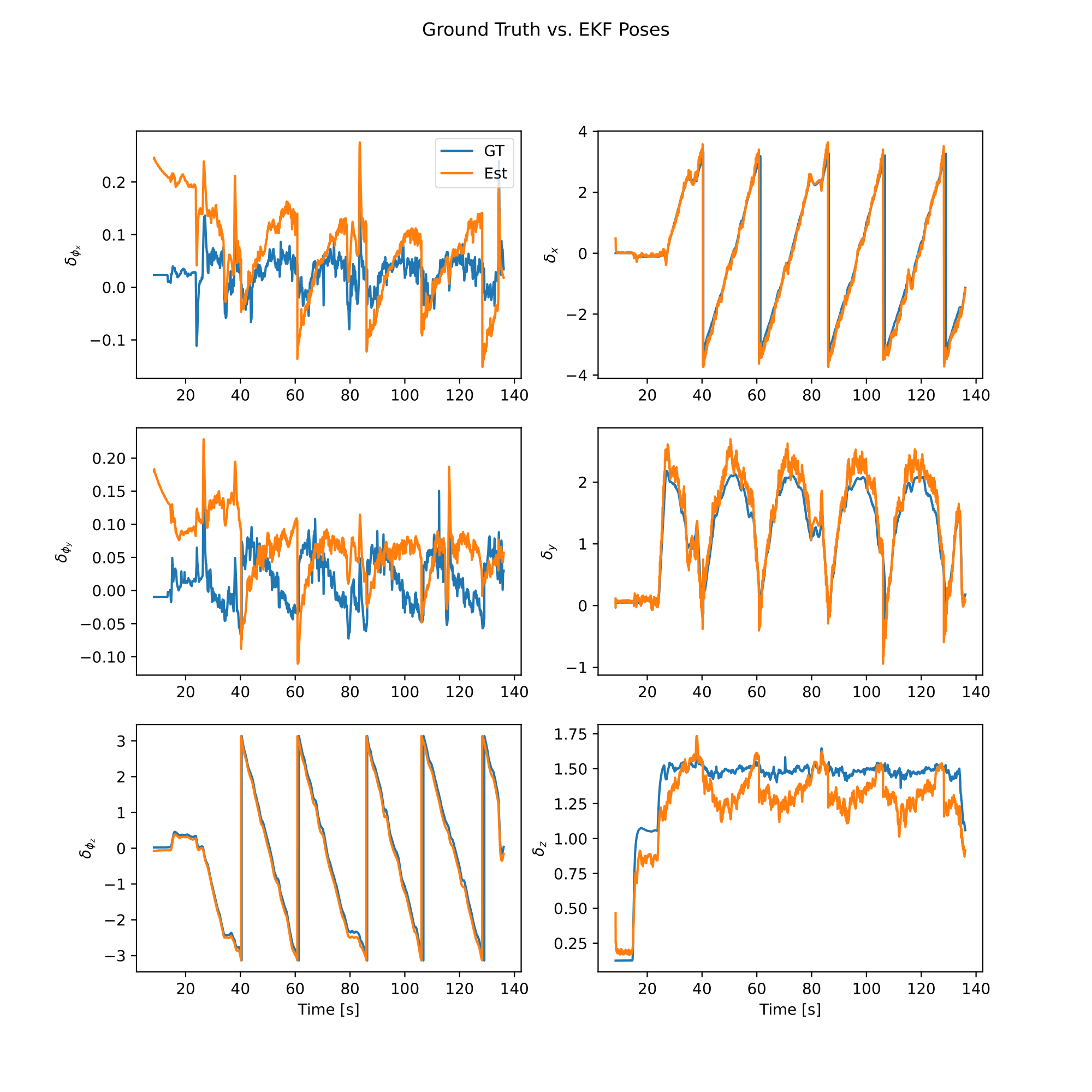
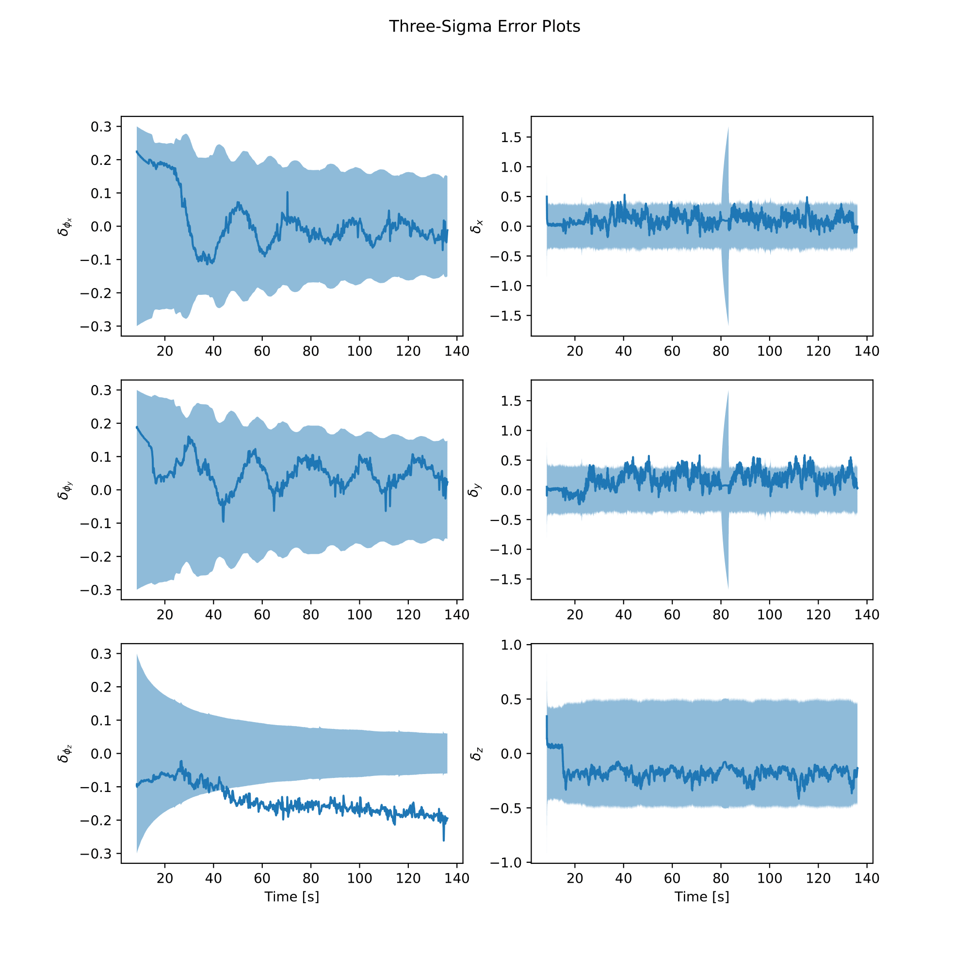
We can now evaluate the EKF using the ground truth data and plot the results. We first evaluate the EKF using the ground truth data and the EKF history, using the example-specific evaluation functions in the models module.
analysis = model.EvaluateEKF(gt_se3, ekf_history, exp_name)
Lastly, we call the following functions to plot the results and save the results to disk, and we are done!
analysis.plot_error()
analysis.plot_poses()
analysis.save_results()
 |  |