$SE_2(3)$ EKF with IMU - Three Robots

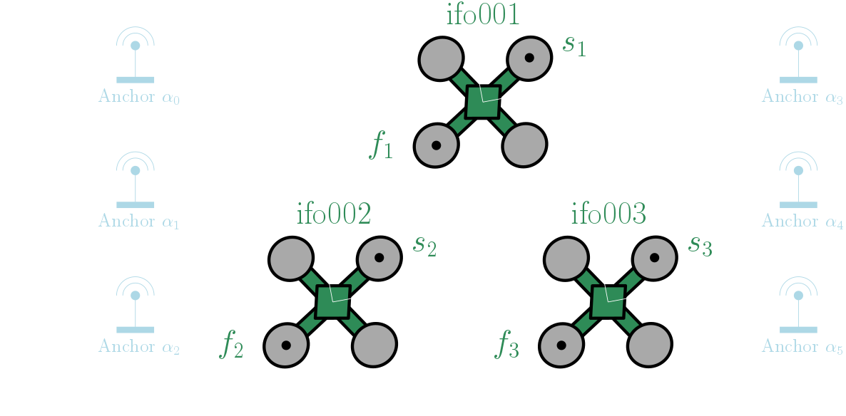
This example shows how we can use MILUV to test out an Extended Kalman Filter (EKF) for three robots using Inertial Measurement Units (IMUs). This extends the one-robot IMU example to three robots, in the same manner we extended the one-robot VINS example to three robots. We will keep this example brief as it is not much different than what we have seen before. The data we use is the same as the one-robot example, but now we also use the inter-robot UWB range data to estimate the poses and IMU biases of all the robots.

Importing Libraries and MILUV Utilities

We start by importing the necessary libraries and utilities for this example as in the VINS example, with the only change being the EKF model we are using.

import numpy as np
import pandas as pd

from miluv.data import DataLoader
import miluv.utils as utils
import examples.ekfutils.imu_three_robots_models as model
import examples.ekfutils.common as common

Loading the Data

We will extract the same data we did for the three-robot VINS example, and merge the UWB range and height data for all the robots.

exp_name = "1c"

miluv = DataLoader(exp_name, imu = "px4", cam = None, mag = False)
data = miluv.data

uwb_range = pd.concat([data[robot]["uwb_range"] for robot in data.keys()])
height = pd.concat([data[robot]["height"].assign(robot=robot) for robot in data.keys()])

We then extract the timestamps where we have UWB range and height data, and sort them in ascending order.

query_timestamps = np.append(uwb_range["timestamp"].to_numpy(), height["timestamp"].to_numpy())
query_timestamps = np.sort(np.unique(query_timestamps))

We then use this to query the IMU data at these timestamps, extracing both the accelerometer and gyroscope data as before, except now we do it for all three robots.

imu_at_query_timestamps = {
    robot: miluv.query_by_timestamps(query_timestamps, robots=robot, sensors="imu_px4")[robot]
    for robot in data.keys()
}
gyro: pd.DataFrame = {
    robot: imu_at_query_timestamps[robot]["imu_px4"][["timestamp", "angular_velocity.x", "angular_velocity.y", "angular_velocity.z"]]
    for robot in data.keys()
}
accel: pd.DataFrame = {
    robot: imu_at_query_timestamps[robot]["imu_px4"][["timestamp", "linear_acceleration.x", "linear_acceleration.y", "linear_acceleration.z"]]
    for robot in data.keys()
}

Lastly, we extract the ground truth poses and biases for all three robots at these timestamps, again taking advantage of the MILUV-provided spline interpolation to get the poses at the query timestamps and get the first derivative of the position to get the velocity.

gt_se23 = {
    robot: utils.get_se23_poses(
        data[robot]["mocap_quat"](query_timestamps), data[robot]["mocap_pos"].derivative(nu=1)(query_timestamps), data[robot]["mocap_pos"](query_timestamps)
    )
    for robot in data.keys()
}
gt_bias = {
    robot: imu_at_query_timestamps[robot]["imu_px4"][[
        "gyro_bias.x", "gyro_bias.y", "gyro_bias.z", 
        "accel_bias.x", "accel_bias.y", "accel_bias.z"
    ]].to_numpy()
    for robot in data.keys()
}

Extended Kalman Filter

The EKF for this example is very similar to the one-robot example, except that now we apply the process model and corrections to all three robots. Additionally, we now have to account for the inter-robot UWB range data. We start by initializing the EKF history for the poses and biases of all three robots.

ekf_history = {
    robot: {
        "pose": common.MatrixStateHistory(state_dim=5, covariance_dim=9),
        "bias": common.VectorStateHistory(state_dim=6)
    }
    for robot in data.keys()
}

We then initialize the EKF with the first ground truth pose, the anchor postions, and UWB tag moment arms.

ekf = model.EKF(
    {robot: gt_se23[robot][0] for robot in data.keys()}, 
    miluv.anchors, 
    miluv.tag_moment_arms
)

The main loop of the EKF is to iterate through the query timestamps and do the prediction and correction steps, which is where the EKF magic happens and is what we will go through next.

for i in range(0, len(query_timestamps)):
    # ----> TODO: Implement the EKF prediction and correction steps

Prediction

The prediction step is exactly the same as in the one-robot example, just doing so for all 3 robots. We first extract the IMU data using

for i in range(0, len(query_timestamps)):
    input = {
        robot: np.array([
            gyro[robot].iloc[i]["angular_velocity.x"], gyro[robot].iloc[i]["angular_velocity.y"], 
            gyro[robot].iloc[i]["angular_velocity.z"], accel[robot].iloc[i]["linear_acceleration.x"], 
            accel[robot].iloc[i]["linear_acceleration.y"], accel[robot].iloc[i]["linear_acceleration.z"]
        ])
        for robot in data.keys()
    }

    # ----> TODO: EKF prediction using the gyro and vins data

Then by implementing the same prediction step as in the one-robot example inside the models module, we can predict the pose and bias of all three robots.

for i in range(0, len(query_timestamps)):
    # .....
    
    # Do an EKF prediction using the gyro and vins data
    dt = (query_timestamps[i] - query_timestamps[i - 1]) if i > 0 else 0
    ekf.predict(input, dt)

Correction

The correction models for the UWB range and height data are almost identical to the VINS EKF example, the only difference being that $\boldsymbol{\Pi}$, $\mathbf{\tilde{r}}_{1}^{\tau_1 1}$, and $\odot$ operator are defined as in the one-robot IMU example.

# Iterate through the query timestamps
for i in range(0, len(query_timestamps)):
    # .....

    # Check if range data is available at this query timestamp, and do an EKF correction
    range_idx = np.where(uwb_range["timestamp"] == query_timestamps[i])[0]
    if len(range_idx) > 0:
        range_data = uwb_range.iloc[range_idx]
        ekf.correct({
            "range": float(range_data["range"].iloc[0]),
            "to_id": int(range_data["to_id"].iloc[0]),
            "from_id": int(range_data["from_id"].iloc[0])
        })

The same goes for the height measurement, and we can correct the EKF using the following snippet.

for i in range(0, len(query_timestamps)):
    # .....

    # Check if height data is available at this query timestamp, and do an EKF correction
    height_idx = np.where(height["timestamp"] == query_timestamps[i])[0]
    if len(height_idx) > 0:
        height_data = height.iloc[height_idx]
        ekf.correct({
            "height": float(height_data["range"].iloc[0]),
            "robot": height_data["robot"].iloc[0]
        })

Lastly, we store the EKF state and covariance at this query timestamp for postprocessing.

for i in range(0, len(query_timestamps)):
    # .....

    # Store the EKF state and covariance at this query timestamp
    for robot in data.keys():
        ekf_history[robot]["pose"].add(query_timestamps[i], ekf.pose[robot], ekf.pose_covariance[robot])
        ekf_history[robot]["bias"].add(query_timestamps[i], ekf.bias[robot], ekf.bias_covariance[robot])

Results

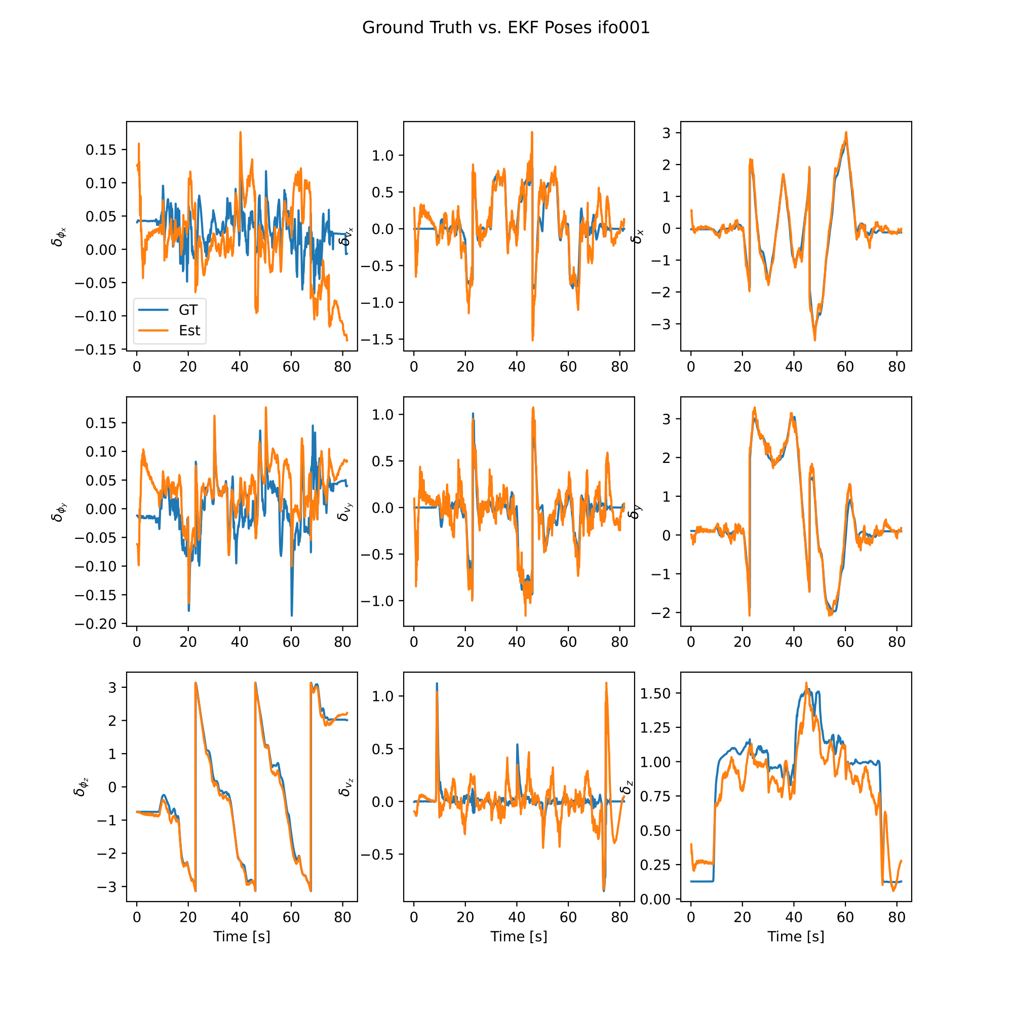
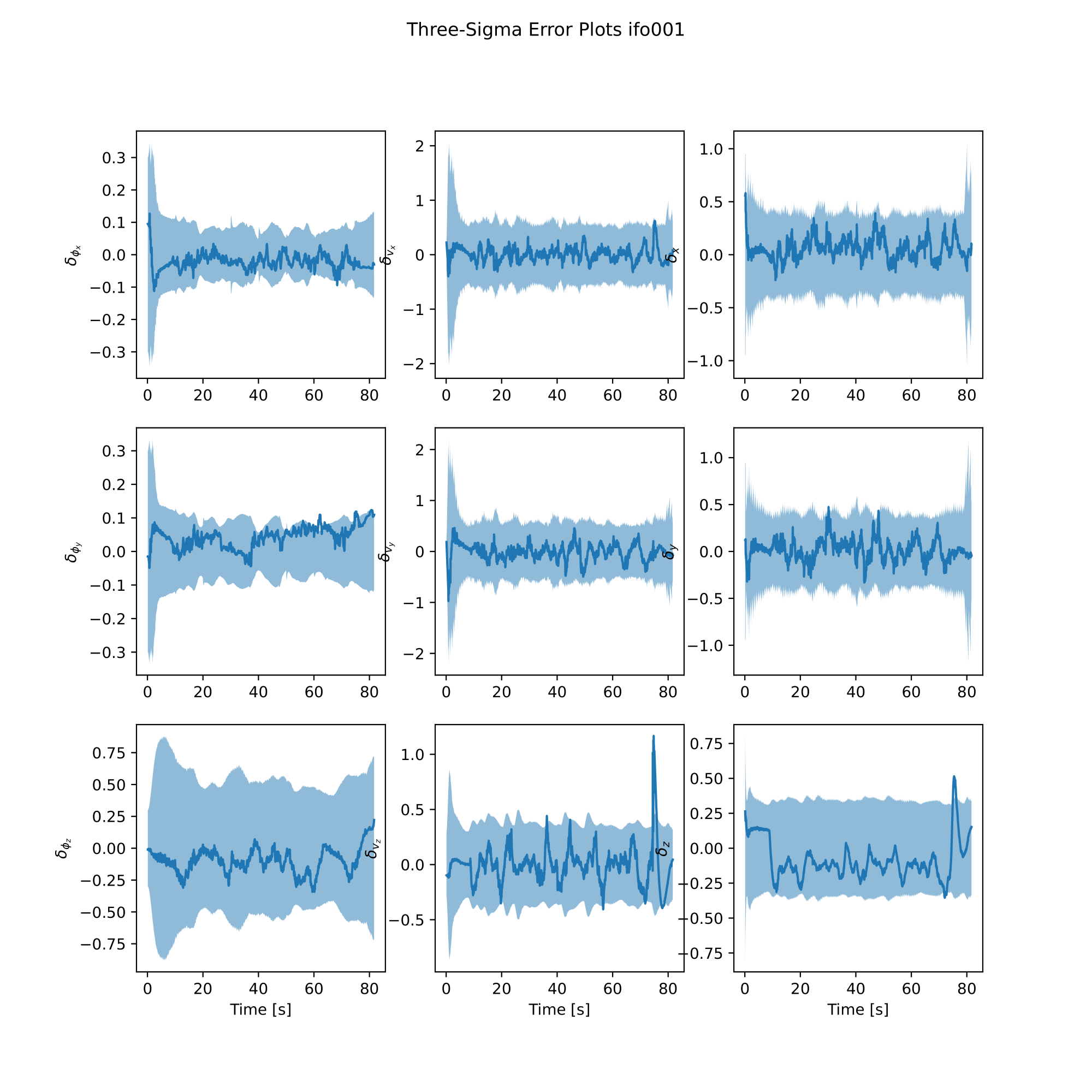
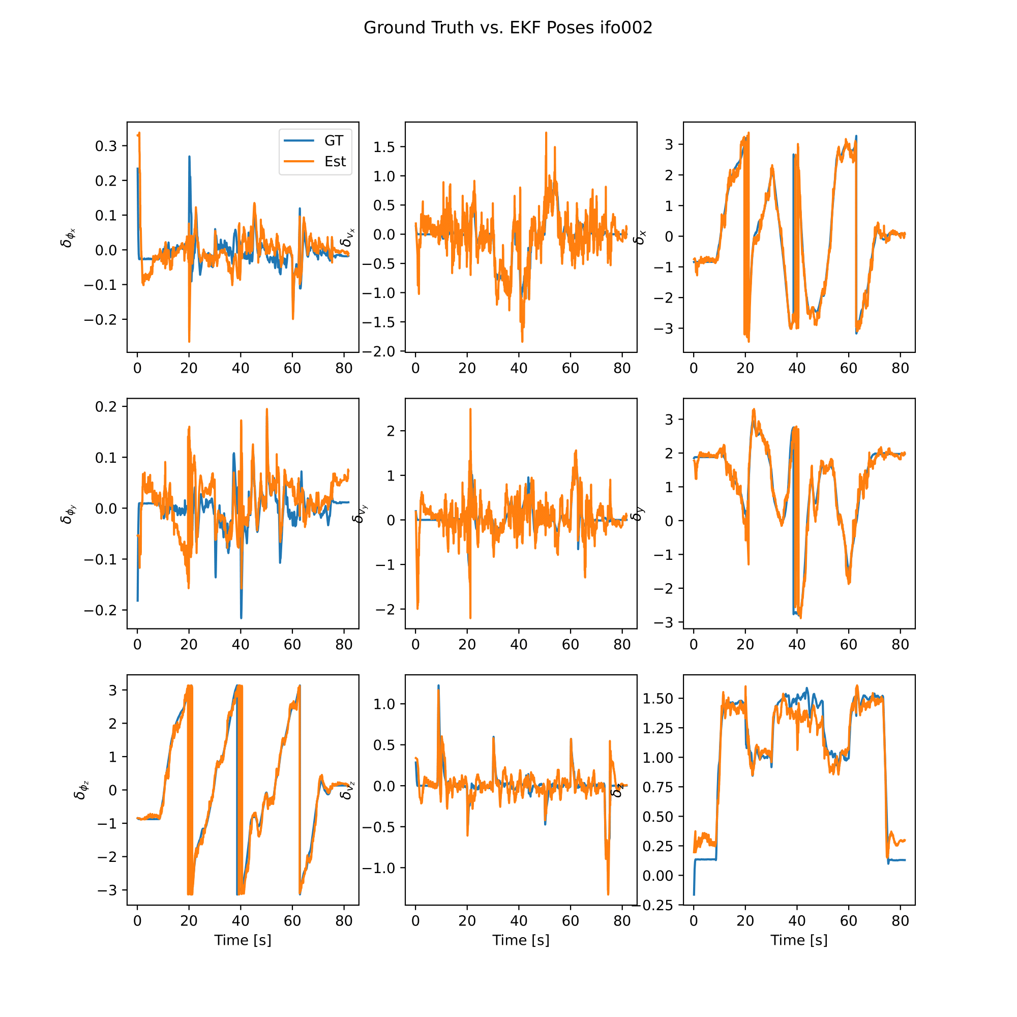
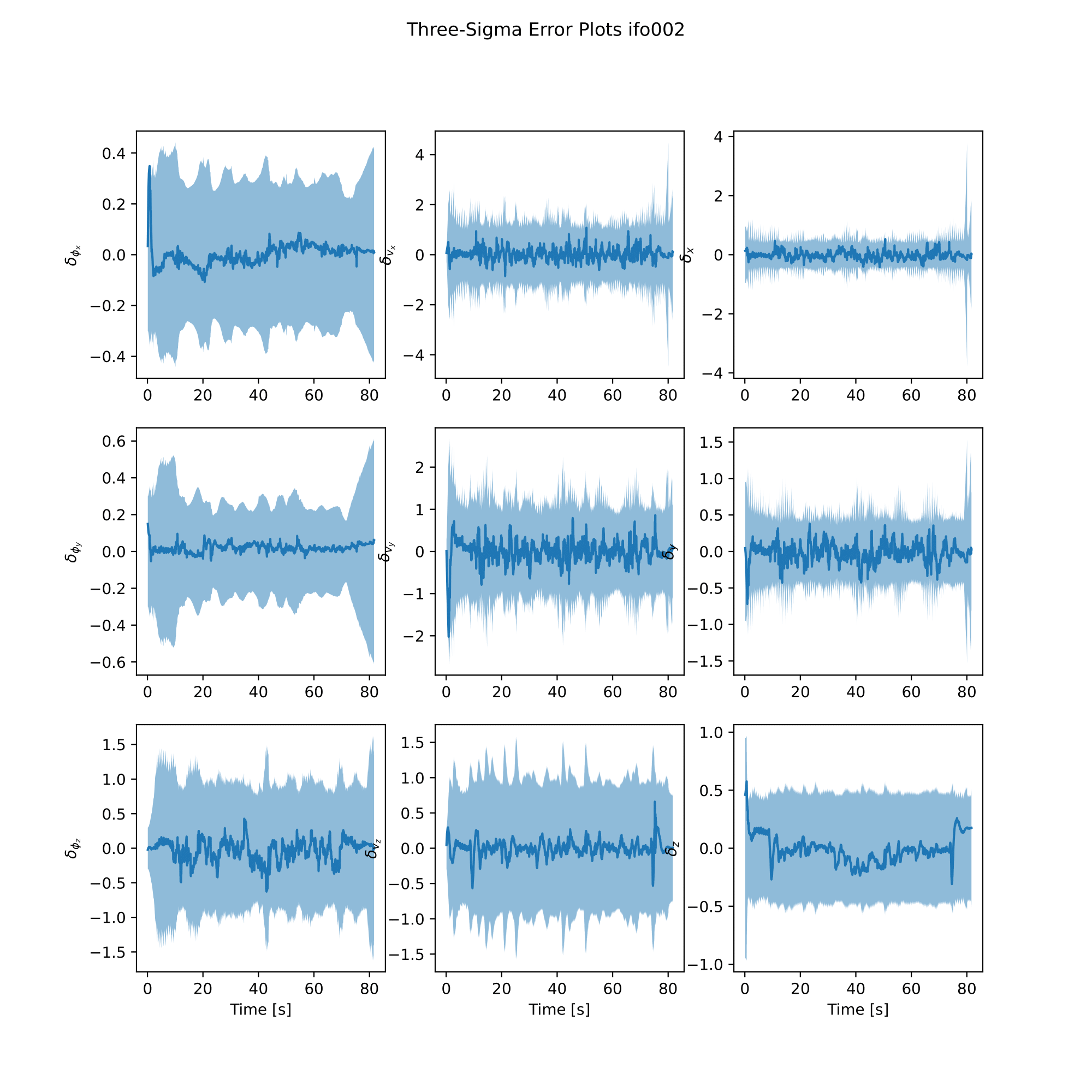
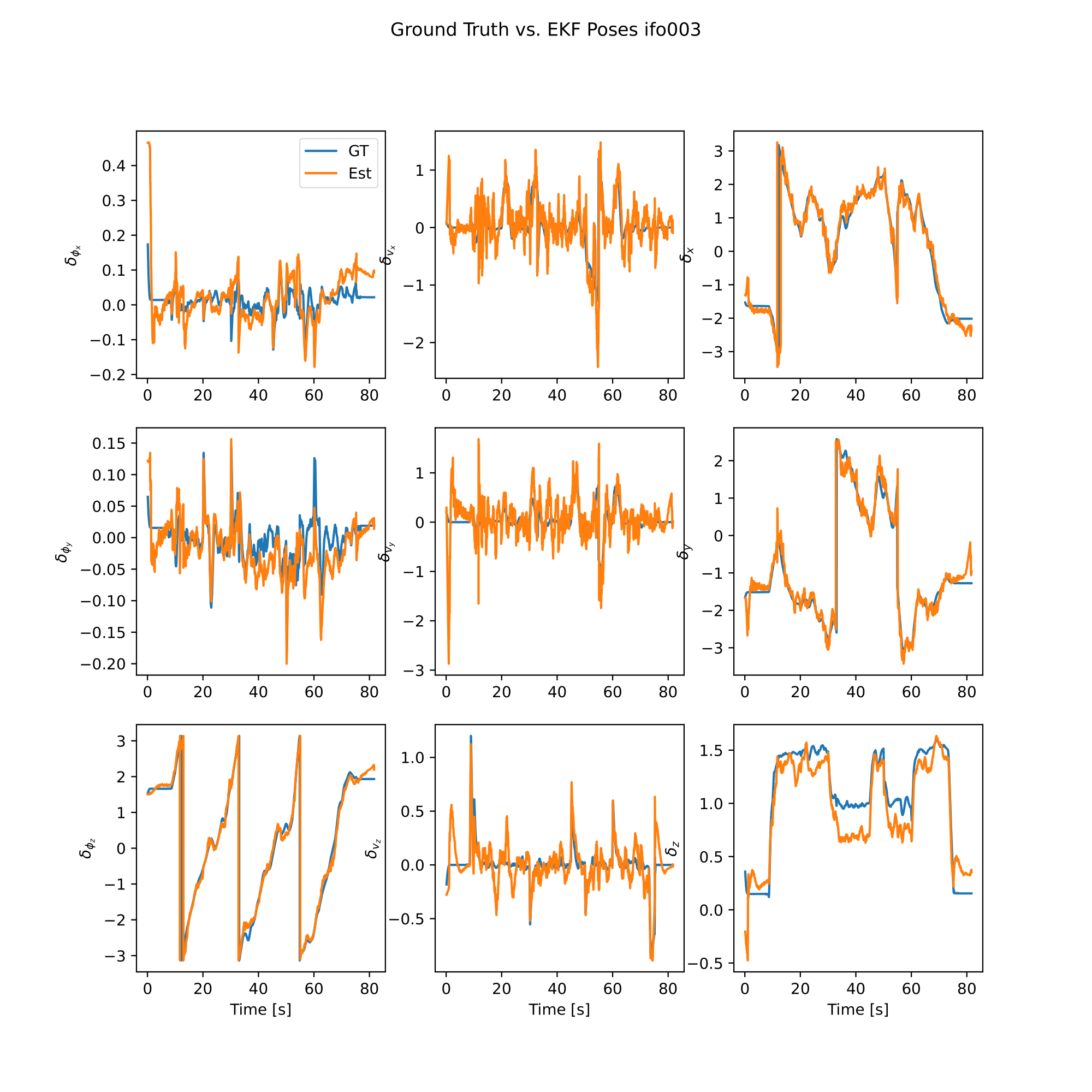
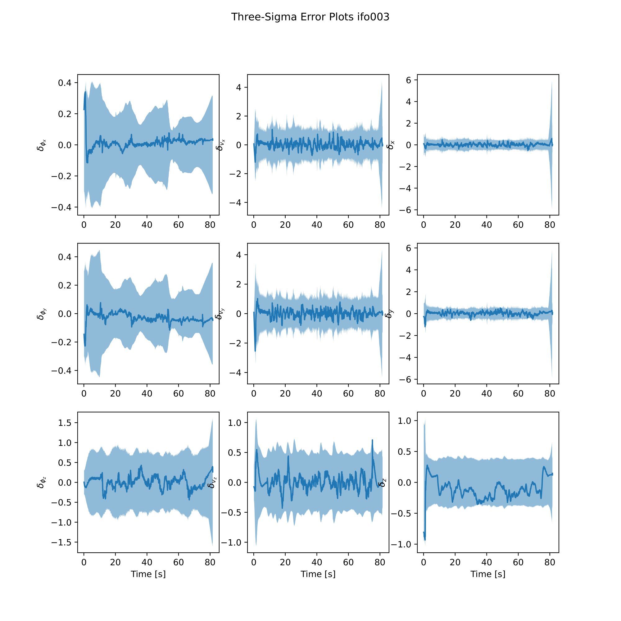
We can now evaluate the EKF using the ground truth data and plot the results. We first evaluate the EKF using the ground truth data and the EKF history, using the example-specific evaluation functions in the models module.

analysis = model.EvaluateEKF(gt_se23, gt_bias, ekf_history, exp_name)

Lastly, we call the following functions to plot the results and save the results to disk, and we are done!

analysis.plot_error()
analysis.plot_poses()
analysis.plot_bias_error()
analysis.save_results()